Euler's formula, named after Leonhard Euler, is a mathematical formula in complex analysis that establishes the fundamental relationship between the trigonometric functions and the complex exponential function. Euler's formula states that, for any real number x, one has where e is the base of the natural logarithm, i is the imaginary unit, and cos and sin are the trigonometric functions cosine and sine respectively. This complex exponential function is sometimes denoted cis x. The formula is still valid if x is a complex number, and is also called Euler's formula in this more general case.
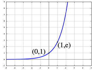
The exponential function is a mathematical function denoted by or . Unless otherwise specified, the term generally refers to the positive-valued function of a real variable, although it can be extended to the complex numbers or generalized to other mathematical objects like matrices or Lie algebras. The exponential function originated from the operation of taking powers of a number, but various modern definitions allow it to be rigorously extended to all real arguments , including irrational numbers. Its ubiquitous occurrence in pure and applied mathematics led mathematician Walter Rudin to consider the exponential function to be "the most important function in mathematics".

In mathematics, the logarithm is the inverse function to exponentiation. That means that the logarithm of a number x to the base b is the exponent to which b must be raised to produce x. For example, since 1000 = 103, the logarithm base of 1000 is 3, or log10 (1000) = 3. The logarithm of x to base b is denoted as logb (x), or without parentheses, logb x. When the base is clear from the context or is irrelevant it is sometimes written log x.

In mathematics, the trigonometric functions are real functions which relate an angle of a right-angled triangle to ratios of two side lengths. They are widely used in all sciences that are related to geometry, such as navigation, solid mechanics, celestial mechanics, geodesy, and many others. They are among the simplest periodic functions, and as such are also widely used for studying periodic phenomena through Fourier analysis.

The Box–Muller transform, by George Edward Pelham Box and Mervin Edgar Muller, is a random number sampling method for generating pairs of independent, standard, normally distributed random numbers, given a source of uniformly distributed random numbers. The method was first mentioned explicitly by Raymond E. A. C. Paley and Norbert Wiener in their 1934 treatise on Fourier transforms in the complex domain. Given the status of these latter authors and the widespread availability and use of their treatise, it is almost certain that Box and Muller were well aware of its contents.
In the mathematical subfields of numerical analysis and mathematical analysis, a trigonometric polynomial is a finite linear combination of functions sin(nx) and cos(nx) with n taking on the values of one or more natural numbers. The coefficients may be taken as real numbers, for real-valued functions. For complex coefficients, there is no difference between such a function and a finite Fourier series.
CORDIC, Volder's algorithm, Digit-by-digit method, Circular CORDIC, Linear CORDIC, Hyperbolic CORDIC, and Generalized Hyperbolic CORDIC, is a simple and efficient algorithm to calculate trigonometric functions, hyperbolic functions, square roots, multiplications, divisions, and exponentials and logarithms with arbitrary base, typically converging with one digit per iteration. CORDIC is therefore also an example of digit-by-digit algorithms. CORDIC and closely related methods known as pseudo-multiplication and pseudo-division or factor combining are commonly used when no hardware multiplier is available, as the only operations they require are additions, subtractions, bitshift and lookup tables. As such, they all belong to the class of shift-and-add algorithms. In computer science, CORDIC is often used to implement floating-point arithmetic when the target platform lacks hardware multiply for cost or space reasons.
In mathematics, trigonometric interpolation is interpolation with trigonometric polynomials. Interpolation is the process of finding a function which goes through some given data points. For trigonometric interpolation, this function has to be a trigonometric polynomial, that is, a sum of sines and cosines of given periods. This form is especially suited for interpolation of periodic functions.
The Pythagorean trigonometric identity, also called simply the Pythagorean identity, is an identity expressing the Pythagorean theorem in terms of trigonometric functions. Along with the sum-of-angles formulae, it is one of the basic relations between the sine and cosine functions.
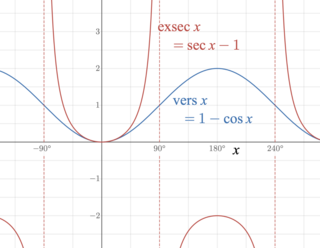
The external secant function is a trigonometric function defined in terms of the secant function:
Prosthaphaeresis was an algorithm used in the late 16th century and early 17th century for approximate multiplication and division using formulas from trigonometry. For the 25 years preceding the invention of the logarithm in 1614, it was the only known generally applicable way of approximating products quickly. Its name comes from the Greek prosthen (πρόσθεν) meaning before and aphaeresis (ἀφαίρεσις), meaning taking away or subtraction.

The small-angle approximations can be used to approximate the values of the main trigonometric functions, provided that the angle in question is small and is measured in radians:
In mathematics, sine and cosine are trigonometric functions of an angle. The sine and cosine of an acute angle are defined in the context of a right triangle: for the specified angle, its sine is the ratio of the length of the side that is opposite that angle to the length of the longest side of the triangle, and the cosine is the ratio of the length of the adjacent leg to that of the hypotenuse. For an angle , the sine and cosine functions are denoted as and .
Early study of triangles can be traced to the 2nd millennium BC, in Egyptian mathematics and Babylonian mathematics. Trigonometry was also prevalent in Kushite mathematics. Systematic study of trigonometric functions began in Hellenistic mathematics, reaching India as part of Hellenistic astronomy. In Indian astronomy, the study of trigonometric functions flourished in the Gupta period, especially due to Aryabhata, who discovered the sine function, cosine function, and versine function.
In mathematics, the values of the trigonometric functions can be expressed approximately, as in , or exactly, as in . While trigonometric tables contain many approximate values, the exact values for certain angles can be expressed by a combination of arithmetic operations and square roots. The angles with trigonometric values that are expressible in this way are exactly those that can be constructed with a compass and straight edge, and the values are called constructible numbers.
Trigonometry is a branch of mathematics concerned with relationships between angles and side lengths of triangles. In particular, the trigonometric functions relate the angles of a right triangle with ratios of its side lengths. The field emerged in the Hellenistic world during the 3rd century BC from applications of geometry to astronomical studies. The Greeks focused on the calculation of chords, while mathematicians in India created the earliest-known tables of values for trigonometric ratios such as sine.
In mathematics, Bhāskara I's sine approximation formula is a rational expression in one variable for the computation of the approximate values of the trigonometric sines discovered by Bhāskara I, a seventh-century Indian mathematician. This formula is given in his treatise titled Mahabhaskariya. It is not known how Bhāskara I arrived at his approximation formula. However, several historians of mathematics have put forward different hypotheses as to the method Bhāskara might have used to arrive at his formula. The formula is elegant and simple, and it enables the computation of reasonably accurate values of trigonometric sines without the use of geometry.

In mathematics, a unit circle is a circle of unit radius—that is, a radius of 1. Frequently, especially in trigonometry, the unit circle is the circle of radius 1 centered at the origin in the Cartesian coordinate system in the Euclidean plane. In topology, it is often denoted as S1 because it is a one-dimensional unit n-sphere.
A system of polynomial equations is a set of simultaneous equations f1 = 0, ..., fh = 0 where the fi are polynomials in several variables, say x1, ..., xn, over some field k.