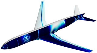
The Navier–Stokes equations are partial differential equations which describe the motion of viscous fluid substances. They were named after French engineer and physicist Claude-Louis Navier and the Irish physicist and mathematician George Gabriel Stokes. They were developed over several decades of progressively building the theories, from 1822 (Navier) to 1842–1850 (Stokes).
In fluid dynamics, turbulence or turbulent flow is fluid motion characterized by chaotic changes in pressure and flow velocity. It is in contrast to a laminar flow, which occurs when a fluid flows in parallel layers, with no disruption between those layers.

In physics and fluid mechanics, a boundary layer is the thin layer of fluid in the immediate vicinity of a bounding surface formed by the fluid flowing along the surface. The fluid's interaction with the wall induces a no-slip boundary condition. The flow velocity then monotonically increases above the surface until it returns to the bulk flow velocity. The thin layer consisting of fluid whose velocity has not yet returned to the bulk flow velocity is called the velocity boundary layer.
The Richardson number (Ri) is named after Lewis Fry Richardson (1881–1953). It is the dimensionless number that expresses the ratio of the buoyancy term to the flow shear term:

The surface layer is the layer of a turbulent fluid most affected by interaction with a solid surface or the surface separating a gas and a liquid where the characteristics of the turbulence depend on distance from the interface. Surface layers are characterized by large normal gradients of tangential velocity and large concentration gradients of any substances transported to or from the interface.
The Reynolds-averaged Navier–Stokes equations are time-averaged equations of motion for fluid flow. The idea behind the equations is Reynolds decomposition, whereby an instantaneous quantity is decomposed into its time-averaged and fluctuating quantities, an idea first proposed by Osborne Reynolds. The RANS equations are primarily used to describe turbulent flows. These equations can be used with approximations based on knowledge of the properties of flow turbulence to give approximate time-averaged solutions to the Navier–Stokes equations. For a stationary flow of an incompressible Newtonian fluid, these equations can be written in Einstein notation in Cartesian coordinates as:

Large eddy simulation (LES) is a mathematical model for turbulence used in computational fluid dynamics. It was initially proposed in 1963 by Joseph Smagorinsky to simulate atmospheric air currents, and first explored by Deardorff (1970). LES is currently applied in a wide variety of engineering applications, including combustion, acoustics, and simulations of the atmospheric boundary layer.
In fluid dynamics, the Reynolds stress is the component of the total stress tensor in a fluid obtained from the averaging operation over the Navier–Stokes equations to account for turbulent fluctuations in fluid momentum.

In fluid dynamics, turbulence modeling is the construction and use of a mathematical model to predict the effects of turbulence. Turbulent flows are commonplace in most real-life scenarios, including the flow of blood through the cardiovascular system, the airflow over an aircraft wing, the re-entry of space vehicles, besides others. In spite of decades of research, there is no analytical theory to predict the evolution of these turbulent flows. The equations governing turbulent flows can only be solved directly for simple cases of flow. For most real-life turbulent flows, CFD simulations use turbulent models to predict the evolution of turbulence. These turbulence models are simplified constitutive equations that predict the statistical evolution of turbulent flows.

In fluid dynamics, eddy diffusion, eddy dispersion, or turbulent diffusion is a process by which fluid substances mix together due to eddy motion. These eddies can vary widely in size, from subtropical ocean gyres down to the small Kolmogorov microscales, and occur as a result of turbulence. The theory of eddy diffusion was first developed by Sir Geoffrey Ingram Taylor.
The turbulent Prandtl number (Prt) is a non-dimensional term defined as the ratio between the momentum eddy diffusivity and the heat transfer eddy diffusivity. It is useful for solving the heat transfer problem of turbulent boundary layer flows. The simplest model for Prt is the Reynolds analogy, which yields a turbulent Prandtl number of 1. From experimental data, Prt has an average value of 0.85, but ranges from 0.7 to 0.9 depending on the Prandtl number of the fluid in question.
Turbulent diffusion is the transport of mass, heat, or momentum within a system due to random and chaotic time dependent motions. It occurs when turbulent fluid systems reach critical conditions in response to shear flow, which results from a combination of steep concentration gradients, density gradients, and high velocities. It occurs much more rapidly than molecular diffusion and is therefore extremely important for problems concerning mixing and transport in systems dealing with combustion, contaminants, dissolved oxygen, and solutions in industry. In these fields, turbulent diffusion acts as an excellent process for quickly reducing the concentrations of a species in a fluid or environment, in cases where this is needed for rapid mixing during processing, or rapid pollutant or contaminant reduction for safety.
In fluid dynamics, the Taylor microscale, which is sometimes called the turbulence length scale, is a length scale used to characterize a turbulent fluid flow. This microscale is named after Geoffrey Ingram Taylor. The Taylor microscale is the intermediate length scale at which fluid viscosity significantly affects the dynamics of turbulent eddies in the flow. This length scale is traditionally applied to turbulent flow which can be characterized by a Kolmogorov spectrum of velocity fluctuations. In such a flow, length scales which are larger than the Taylor microscale are not strongly affected by viscosity. These larger length scales in the flow are generally referred to as the inertial range. Below the Taylor microscale the turbulent motions are subject to strong viscous forces and kinetic energy is dissipated into heat. These shorter length scale motions are generally termed the dissipation range.

In fluid dynamics, the radiation stress is the depth-integrated – and thereafter phase-averaged – excess momentum flux caused by the presence of the surface gravity waves, which is exerted on the mean flow. The radiation stresses behave as a second-order tensor.
K-epsilon (k-ε) turbulence model is one of the most common models used in computational fluid dynamics (CFD) to simulate mean flow characteristics for turbulent flow conditions. It is a two equation model that gives a general description of turbulence by means of two transport equations. The original impetus for the K-epsilon model was to improve the mixing-length model, as well as to find an alternative to algebraically prescribing turbulent length scales in moderate to high complexity flows.
Reynolds stress equation model (RSM), also referred to as second moment closures are the most complete classical turbulence model. In these models, the eddy-viscosity hypothesis is avoided and the individual components of the Reynolds stress tensor are directly computed. These models use the exact Reynolds stress transport equation for their formulation. They account for the directional effects of the Reynolds stresses and the complex interactions in turbulent flows. Reynolds stress models offer significantly better accuracy than eddy-viscosity based turbulence models, while being computationally cheaper than Direct Numerical Simulations (DNS) and Large Eddy Simulations.
In computational fluid dynamics, the k–omega (k–ω) turbulence model is a common two-equation turbulence model, that is used as an approximation for the Reynolds-averaged Navier–Stokes equations (RANS equations). The model attempts to predict turbulence by two partial differential equations for two variables, k and ω, with the first variable being the turbulence kinetic energy (k) while the second (ω) is the specific rate of dissipation (of the turbulence kinetic energy k into internal thermal energy).
Menter's Shear Stress Transport turbulence model, or SST, is a widely used and robust two-equation eddy-viscosity turbulence model used in Computational Fluid Dynamics. The model combines the k-omega turbulence model and K-epsilon turbulence model such that the k-omega is used in the inner region of the boundary layer and switches to the k-epsilon in the free shear flow.

Gamma-Re (γ-Re) transition model is a two equation model used in Computational Fluid Dynamics (CFD) to modify turbulent transport equations to simulate laminar, laminar-to-turbulent and turbulence states in a fluid flow. The Gamma-Re model does not intend to model the physics of the problem but attempts to fit a wide range of experiments and transition methods into its formulation. The transition model calculated an intermittency factor that creates turbulence by slowly introducing turbulent production at the laminar-to-turbulent transition location.

In continuum mechanics, an energy cascade involves the transfer of energy from large scales of motion to the small scales or a transfer of energy from the small scales to the large scales. This transfer of energy between different scales requires that the dynamics of the system is nonlinear. Strictly speaking, a cascade requires the energy transfer to be local in scale, evoking a cascading waterfall from pool to pool without long-range transfers across the scale domain.


