
In vector calculus, divergence is a vector operator that operates on a vector field, producing a scalar field giving the quantity of the vector field's source at each point. More technically, the divergence represents the volume density of the outward flux of a vector field from an infinitesimal volume around a given point.
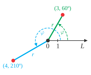
In mathematics, the polar coordinate system is a two-dimensional coordinate system in which each point on a plane is determined by a distance from a reference point and an angle from a reference direction. The reference point is called the pole, and the ray from the pole in the reference direction is the polar axis. The distance from the pole is called the radial coordinate, radial distance or simply radius, and the angle is called the angular coordinate, polar angle, or azimuth. Angles in polar notation are generally expressed in either degrees or radians.

In mathematics, a spherical coordinate system is a coordinate system for three-dimensional space where the position of a point is specified by three numbers: the radial distance of that point from a fixed origin, its polar angle measured from a fixed zenith direction, and the azimuthal angle of its orthogonal projection on a reference plane that passes through the origin and is orthogonal to the zenith, measured from a fixed reference direction on that plane. It can be seen as the three-dimensional version of the polar coordinate system.

In mathematics and physics, Laplace's equation is a second-order partial differential equation named after Pierre-Simon Laplace, who first studied its properties. This is often written as

The Navier–Stokes equations are partial differential equations which describe the motion of viscous fluid substances, named after French engineer and physicist Claude-Louis Navier and Anglo-Irish physicist and mathematician George Gabriel Stokes. They were developed over several decades of progressively building the theories, from 1822 (Navier) to 1842-1850 (Stokes).
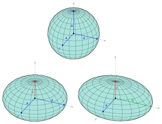
An ellipsoid is a surface that may be obtained from a sphere by deforming it by means of directional scalings, or more generally, of an affine transformation.
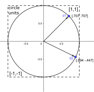
In mathematics, a unit vector in a normed vector space is a vector of length 1. A unit vector is often denoted by a lowercase letter with a circumflex, or "hat", as in .
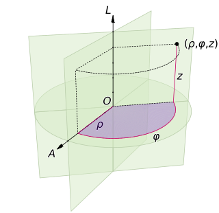
A cylindrical coordinate system is a three-dimensional coordinate system that specifies point positions by the distance from a chosen reference axis (axis L in the image opposite), the direction from the axis relative to a chosen reference direction (axis A), and the distance from a chosen reference plane perpendicular to the axis (plane containing the purple section). The latter distance is given as a positive or negative number depending on which side of the reference plane faces the point.
In calculus, integration by substitution, also known as u-substitution, reverse chain rule or change of variables, is a method for evaluating integrals and antiderivatives. It is the counterpart to the chain rule for differentiation, and can loosely be thought of as using the chain rule "backwards".
In vector calculus, the Jacobian matrix of a vector-valued function of several variables is the matrix of all its first-order partial derivatives. When this matrix is square, that is, when the function takes the same number of variables as input as the number of vector components of its output, its determinant is referred to as the Jacobian determinant. Both the matrix and the determinant are often referred to simply as the Jacobian in literature.

In applied mechanics, bending characterizes the behavior of a slender structural element subjected to an external load applied perpendicularly to a longitudinal axis of the element.

In mathematics (specifically multivariable calculus), a multiple integral is a definite integral of a function of several real variables, for instance, f(x, y) or f(x, y, z). Integrals of a function of two variables over a region in (the real-number plane) are called double integrals, and integrals of a function of three variables over a region in (real-number 3D space) are called triple integrals. For multiple integrals of a single-variable function, see the Cauchy formula for repeated integration.
The Mason–Weaver equation describes the sedimentation and diffusion of solutes under a uniform force, usually a gravitational field. Assuming that the gravitational field is aligned in the z direction, the Mason–Weaver equation may be written

Toroidal coordinates are a three-dimensional orthogonal coordinate system that results from rotating the two-dimensional bipolar coordinate system about the axis that separates its two foci. Thus, the two foci and in bipolar coordinates become a ring of radius in the plane of the toroidal coordinate system; the -axis is the axis of rotation. The focal ring is also known as the reference circle.

Oblate spheroidal coordinates are a three-dimensional orthogonal coordinate system that results from rotating the two-dimensional elliptic coordinate system about the non-focal axis of the ellipse, i.e., the symmetry axis that separates the foci. Thus, the two foci are transformed into a ring of radius in the x-y plane. Oblate spheroidal coordinates can also be considered as a limiting case of ellipsoidal coordinates in which the two largest semi-axes are equal in length.
In mathematics, the cylindrical harmonics are a set of linearly independent functions that are solutions to Laplace's differential equation, , expressed in cylindrical coordinates, ρ (radial coordinate), φ (polar angle), and z (height). Each function Vn(k) is the product of three terms, each depending on one coordinate alone. The ρ-dependent term is given by Bessel functions (which occasionally are also called cylindrical harmonics).
In mathematics, the spectral theory of ordinary differential equations is the part of spectral theory concerned with the determination of the spectrum and eigenfunction expansion associated with a linear ordinary differential equation. In his dissertation Hermann Weyl generalized the classical Sturm–Liouville theory on a finite closed interval to second order differential operators with singularities at the endpoints of the interval, possibly semi-infinite or infinite. Unlike the classical case, the spectrum may no longer consist of just a countable set of eigenvalues, but may also contain a continuous part. In this case the eigenfunction expansion involves an integral over the continuous part with respect to a spectral measure, given by the Titchmarsh–Kodaira formula. The theory was put in its final simplified form for singular differential equations of even degree by Kodaira and others, using von Neumann's spectral theorem. It has had important applications in quantum mechanics, operator theory and harmonic analysis on semisimple Lie groups.
The Mehler kernel is a complex-valued function found to be the propagator of the quantum harmonic oscillator.
Lagrangian field theory is a formalism in classical field theory. It is the field-theoretic analogue of Lagrangian mechanics. Lagrangian mechanics is used to analyze the motion of a system of discrete particles each with a finite number of degrees of freedom. Lagrangian field theory applies to continua and fields, which have an infinite number of degrees of freedom.


