Algorithmic inference

Algorithmic inference gathers new developments in the statistical inference methods made feasible by the powerful computing devices widely available to any data analyst. Cornerstones in this field are computational learning theory, granular computing, bioinformatics, and, long ago, structural probability ( Fraser 1966 ). The main focus is on the algorithms which compute statistics rooting the study of a random phenomenon, along with the amount of data they must feed on to produce reliable results. This shifts the interest of mathematicians from the study of the distribution laws to the functional properties of the statistics, and the interest of computer scientists from the algorithms for processing data to the information they process.

The Fisher parametric inference problem

Concerning the identification of the parameters of a distribution law, the mature reader may recall lengthy disputes in the mid 20th century about the interpretation of their variability in terms of fiducial distribution ( Fisher 1956 ), structural probabilities ( Fraser 1966 ), priors/posteriors ( Ramsey 1925 ), and so on. From an epistemology viewpoint, this entailed a companion dispute as to the nature of probability: is it a physical feature of phenomena to be described through random variables or a way of synthesizing data about a phenomenon? Opting for the latter, Fisher defines a fiducial distribution law of parameters of a given random variable that he deduces from a sample of its specifications. With this law he computes, for instance "the probability that μ (mean of a Gaussian variable – omeur note) is less than any assigned value, or the probability that it lies between any assigned values, or, in short, its probability distribution, in the light of the sample observed".

The classic solution

Fisher fought hard to defend the difference and superiority of his notion of parameter distribution in comparison to analogous notions, such as Bayes' posterior distribution, Fraser's constructive probability and Neyman's confidence intervals. For half a century, Neyman's confidence intervals won out for all practical purposes, crediting the phenomenological nature of probability. With this perspective, when you deal with a Gaussian variable, its mean μ is fixed by the physical features of the phenomenon you are observing, where the observations are random operators, hence the observed values are specifications of a random sample. Because of their randomness, you may compute from the sample specific intervals containing the fixed μ with a given probability that you denote confidence.

Example

Let X be a Gaussian variable ^[1] with parameters ${\displaystyle \mu }$ and ${\displaystyle \sigma ^{2}}$ and ${\displaystyle \{X_{1},\ldots ,X_{m}\}}$ a sample drawn from it. Working with statistics

${\displaystyle S_{\mu }=\sum _{i=1}^{m}X_{i}}$

and

${\displaystyle S_{\sigma ^{2}}=\sum _{i=1}^{m}(X_{i}-{\overline {X}})^{2},{\text{ where }}{\overline {X}}={\frac {S_{\mu }}{m}}}$

is the sample mean, we recognize that

${\displaystyle T={\frac {S_{\mu }-m\mu }{\sqrt {S_{\sigma ^{2}}}}}{\sqrt {\frac {m-1}{m}}}={\frac {{\overline {X}}-\mu }{\sqrt {S_{\sigma ^{2}}/(m(m-1))}}}}$

follows a Student's t distribution ( Wilks 1962 ) with parameter (degrees of freedom) m − 1, so that

${\displaystyle f_{T}(t)={\frac {\Gamma (m/2)}{\Gamma ((m-1)/2)}}{\frac {1}{\sqrt {\pi (m-1)}}}\left(1+{\frac {t^{2}}{m-1}}\right)^{m/2}.}$

Gauging T between two quantiles and inverting its expression as a function of ${\displaystyle \mu }$ you obtain confidence intervals for ${\displaystyle \mu }$.

With the sample specification:

${\displaystyle \mathbf {x} =\{7.14,6.3,3.9,6.46,0.2,2.94,4.14,4.69,6.02,1.58\}}$

having size m = 10, you compute the statistics ${\displaystyle s_{\mu }=43.37}$ and ${\displaystyle s_{\sigma ^{2}}=46.07}$, and obtain a 0.90 confidence interval for ${\displaystyle \mu }$ with extremes (3.03, 5.65).

Inferring functions with the help of a computer

From a modeling perspective the entire dispute looks like a chicken-egg dilemma: either fixed data by first and probability distribution of their properties as a consequence, or fixed properties by first and probability distribution of the observed data as a corollary. The classic solution has one benefit and one drawback. The former was appreciated particularly back when people still did computations with sheet and pencil. Per se, the task of computing a Neyman confidence interval for the fixed parameter θ is hard: you do not know θ, but you look for disposing around it an interval with a possibly very low probability of failing. The analytical solution is allowed for a very limited number of theoretical cases. Vice versa a large variety of instances may be quickly solved in an approximate way via the central limit theorem in terms of confidence interval around a Gaussian distribution – that's the benefit. The drawback is that the central limit theorem is applicable when the sample size is sufficiently large. Therefore, it is less and less applicable with the sample involved in modern inference instances. The fault is not in the sample size on its own part. Rather, this size is not sufficiently large because of the complexity of the inference problem.

With the availability of large computing facilities, scientists refocused from isolated parameters inference to complex functions inference, i.e. re sets of highly nested parameters identifying functions. In these cases we speak about learning of functions (in terms for instance of regression, neuro-fuzzy system or computational learning) on the basis of highly informative samples. A first effect of having a complex structure linking data is the reduction of the number of sample degrees of freedom, i.e. the burning of a part of sample points, so that the effective sample size to be considered in the central limit theorem is too small. Focusing on the sample size ensuring a limited learning error with a given confidence level, the consequence is that the lower bound on this size grows with complexity indices such as VC dimension or detail of a class to which the function we want to learn belongs.

Example

A sample of 1,000 independent bits is enough to ensure an absolute error of at most 0.081 on the estimation of the parameter p of the underlying Bernoulli variable with a confidence of at least 0.99. The same size cannot guarantee a threshold less than 0.088 with the same confidence 0.99 when the error is identified with the probability that a 20-year-old man living in New York does not fit the ranges of height, weight and waistline observed on 1,000 Big Apple inhabitants. The accuracy shortage occurs because both the VC dimension and the detail of the class of parallelepipeds, among which the one observed from the 1,000 inhabitants' ranges falls, are equal to 6.

The general inversion problem solving the Fisher question

With insufficiently large samples, the approach: fixed sample – random properties suggests inference procedures in three steps:

1.	Sampling mechanism. It consists of a pair ${\displaystyle (Z,g_{\boldsymbol {\theta }})}$, where the seed Z is a random variable without unknown parameters, while the explaining function ${\displaystyle g_{\boldsymbol {\theta }}}$ is a function mapping from samples of Z to samples of the random variable X we are interested in. The parameter vector ${\displaystyle {\boldsymbol {\theta }}}$ is a specification of the random parameter ${\displaystyle \mathbf {\Theta } }$. Its components are the parameters of the X distribution law. The Integral Transform Theorem ensures the existence of such a mechanism for each (scalar or vector) X when the seed coincides with the random variable U uniformly distributed in ${\displaystyle [0,1]}$. Example. For X following a Pareto distribution with parameters a and k, i.e. ${\displaystyle F_{X}(x)=\left(1-{\frac {k}{x}}^{a}\right)I_{[k,\infty )}(x),}$ a sampling mechanism ${\displaystyle (U,g_{(a,k)})}$ for X with seed U reads: ${\displaystyle g_{(a,k)}(u)=k(1-u)^{-{\frac {1}{a}}},}$ or, equivalently, ${\displaystyle g_{(a,k)}(u)=ku^{-1/a}.}$
2.	Master equations. The actual connection between the model and the observed data is tossed in terms of a set of relations between statistics on the data and unknown parameters that come as a corollary of the sampling mechanisms. We call these relations master equations. Pivoting around the statistic ${\displaystyle s=h(x_{1},\ldots ,x_{m})=h(g_{\boldsymbol {\theta }}(z_{1}),\ldots ,g_{\boldsymbol {\theta }}(z_{m}))}$, the general form of a master equation is: ${\displaystyle s=\rho ({\boldsymbol {\theta }};z_{1},\ldots ,z_{m})}$. 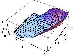With these relations we may inspect the values of the parameters that could have generated a sample with the observed statistic from a particular setting of the seeds representing the seed of the sample. Hence, to the population of sample seeds corresponds a population of parameters. In order to ensure this population clean properties, it is enough to draw randomly the seed values and involve either sufficient statistics or, simply, well-behaved statistics w.r.t. the parameters, in the master equations. For example, the statistics ${\displaystyle s_{1}=\sum _{i=1}^{m}\log x_{i}}$ and ${\displaystyle s_{2}=\min _{i=1,\ldots ,m}\{x_{i}\}}$ prove to be sufficient for parameters a and k of a Pareto random variable X. Thanks to the (equivalent form of the) sampling mechanism ${\displaystyle g_{(a,k)}}$ we may read them as ${\displaystyle s_{1}=m\log k+1/a\sum _{i=1}^{m}\log u_{i}}$ ${\displaystyle s_{2}=\min _{i=1,\ldots ,m}\{ku_{i}^{-{\frac {1}{a}}}\},}$ respectively.
3.	Parameter population. Having fixed a set of master equations, you may map sample seeds into parameters either numerically through a population bootstrap, or analytically through a twisting argument. Hence from a population of seeds you obtain a population of parameters. Example. From the above master equation we can draw a pair of parameters, ${\displaystyle (a,k)}$, compatible with the observed sample by solving the following system of equations: ${\displaystyle a={\frac {\sum \log u_{i}-m\log \min\{u_{i}\}}{s_{1}-m\log s_{2}}}.}$ ${\displaystyle k=\mathrm {e} ^{\frac {as_{1}-\sum \log u_{i}}{ma}}}$ where ${\displaystyle s_{1}}$ and ${\displaystyle s_{2}}$ are the observed statistics and ${\displaystyle u_{1},\ldots ,u_{m}}$ a set of uniform seeds. Transferring to the parameters the probability (density) affecting the seeds, you obtain the distribution law of the random parameters A and K compatible with the statistics you have observed. Compatibility denotes parameters of compatible populations, i.e. of populations that could have generated a sample giving rise to the observed statistics. You may formalize this notion as follows:

Definition

For a random variable and a sample drawn from it a compatible distribution is a distribution having the same sampling mechanism ${\displaystyle {\mathcal {M}}_{X}=(Z,g_{\boldsymbol {\theta }})}$ of X with a value ${\displaystyle {\boldsymbol {\theta }}}$ of the random parameter ${\displaystyle \mathbf {\Theta } }$ derived from a master equation rooted on a well-behaved statistic s.

Example

Joint empirical cumulative distribution function of parameters ${\displaystyle (A,K)}$ of a Pareto random variable.

Cumulative distribution function of the mean M of a Gaussian random variable

You may find the distribution law of the Pareto parameters A and K as an implementation example of the population bootstrap  method as in the figure on the left.

Implementing the twisting argument  method, you get the distribution law ${\displaystyle F_{M}(\mu )}$ of the mean M of a Gaussian variable X on the basis of the statistic ${\displaystyle s_{M}=\sum _{i=1}^{m}x_{i}}$ when ${\displaystyle \Sigma ^{2}}$ is known to be equal to ${\displaystyle \sigma ^{2}}$ ( Apolloni, Malchiodi & Gaito 2006 ). Its expression is:

${\displaystyle F_{M}(\mu )=\Phi \left({\frac {m\mu -s_{M}}{\sigma {\sqrt {m}}}}\right),}$

shown in the figure on the right, where ${\displaystyle \Phi }$ is the cumulative distribution function of a standard normal distribution.

Upper (purple curve) and lower (blue curve) extremes of a 90% confidence interval of the mean M of a Gaussian random variable for a fixed ${\displaystyle \sigma }$ and different values of the statistic s_m.

Computing a confidence interval  for M given its distribution function is straightforward: we need only find two quantiles (for instance ${\displaystyle \delta /2}$ and ${\displaystyle 1-\delta /2}$ quantiles in case we are interested in a confidence interval of level δ symmetric in the tail's probabilities) as indicated on the left in the diagram showing the behavior of the two bounds for different values of the statistic s_m.

The Achilles heel of Fisher's approach lies in the joint distribution of more than one parameter, say mean and variance of a Gaussian distribution. On the contrary, with the last approach (and above-mentioned methods: population bootstrap and twisting argument) we may learn the joint distribution of many parameters. For instance, focusing on the distribution of two or many more parameters, in the figures below we report two confidence regions where the function to be learnt falls with a confidence of 90%. The former concerns the probability with which an extended support vector machine attributes a binary label 1 to the points of the ${\displaystyle (x,y)}$ plane. The two surfaces are drawn on the basis of a set of sample points in turn labelled according to a specific distribution law ( Apolloni et al. 2008 ). The latter concerns the confidence region of the hazard rate of breast cancer recurrence computed from a censored sample ( Apolloni, Malchiodi & Gaito 2006 ).

90% confidence region for the family of support vector machines endowed with hyperbolic tangent profile function

90% confidence region for the hazard function of breast cancer recurrence computed from the censored sample ${\displaystyle t=(9,13,>13,18,12,23,31,34,>45,48,>161),\,}$ with > t denoting a censored time

Notes

1. By default, capital letters (such as U, X) will denote random variables and small letters (u, x) their corresponding specifications.

References

• Fraser, D. A. S. (1966), "Structural probability and generalization", Biometrika, 53 (1/2): 1–9, doi:10.2307/2334048, JSTOR   2334048.
• Fisher, M. A. (1956), Statistical Methods and Scientific Inference, Edinburgh and London: Oliver and Boyd
• Apolloni, B.; Malchiodi, D.; Gaito, S. (2006), Algorithmic Inference in Machine Learning, International Series on Advanced Intelligence, vol. 5 (2nd ed.), Adelaide: Magill, Advanced Knowledge International
• Apolloni, B.; Bassis, S.; Malchiodi, D.; Witold, P. (2008), The Puzzle of Granular Computing, Studies in Computational Intelligence, vol. 138, Berlin: Springer, ISBN   9783540798637
• Ramsey, F. P. (1925), "The Foundations of Mathematics", Proceedings of the London Mathematical Society: 338–384, doi:10.1112/plms/s2-25.1.338.
• Wilks, S.S. (1962), Mathematical Statistics, Wiley Publications in Statistics, New York: John Wiley