Pareto distribution

Pareto Type I

Probability density function Pareto Type I probability density functions for various ${\displaystyle \alpha }$ with ${\displaystyle x_{\mathrm {m} }=1.}$ As ${\displaystyle \alpha \rightarrow \infty ,}$ the distribution approaches ${\displaystyle \delta (x-x_{\mathrm {m} }),}$ where ${\displaystyle \delta }$ is the Dirac delta function.
Cumulative distribution function Pareto Type I cumulative distribution functions for various ${\displaystyle \alpha }$ with ${\displaystyle x_{\mathrm {m} }=1.}$
Parameters	${\displaystyle x_{\mathrm {m} }>0}$ scale (real) ${\displaystyle \alpha >0}$ shape (real)
Support	${\displaystyle x\in [x_{\mathrm {m} },\infty )}$
PDF	${\displaystyle {\frac {\alpha x_{\mathrm {m} }^{\alpha }}{x^{\alpha +1}}}}$
CDF	${\displaystyle 1-\left({\frac {x_{\mathrm {m} }}{x}}\right)^{\alpha }}$
Quantile	${\displaystyle x_{\mathrm {m} }{(1-p)}^{-{\frac {1}{\alpha }}}}$
Mean	${\displaystyle {\begin{cases}\infty &{\text{for }}\alpha \leq 1\\{\dfrac {\alpha x_{\mathrm {m} }}{\alpha -1}}&{\text{for }}\alpha >1\end{cases}}}$
Median	${\displaystyle x_{\mathrm {m} }{\sqrt[{\alpha }]{2}}}$
Mode	${\displaystyle x_{\mathrm {m} }}$
Variance	${\displaystyle {\begin{cases}\infty &{\text{for }}\alpha \leq 2\\{\dfrac {x_{\mathrm {m} }^{2}\alpha }{(\alpha -1)^{2}(\alpha -2)}}&{\text{for }}\alpha >2\end{cases}}}$
Skewness	${\displaystyle {\frac {2(1+\alpha )}{\alpha -3}}{\sqrt {\frac {\alpha -2}{\alpha }}}{\text{ for }}\alpha >3}$
Excess kurtosis	${\displaystyle {\frac {6(\alpha ^{3}+\alpha ^{2}-6\alpha -2)}{\alpha (\alpha -3)(\alpha -4)}}{\text{ for }}\alpha >4}$
Entropy	${\displaystyle \log \left(\left({\frac {x_{\mathrm {m} }}{\alpha }}\right)\,e^{1+{\tfrac {1}{\alpha }}}\right)}$
MGF	does not exist
CF	${\displaystyle \alpha (-ix_{\mathrm {m} }t)^{\alpha }\Gamma (-\alpha ,-ix_{\mathrm {m} }t)}$
Fisher information	${\displaystyle {\mathcal {I}}(x_{\mathrm {m} },\alpha )={\begin{bmatrix}{\dfrac {\alpha ^{2}}{x_{\mathrm {m} }^{2}}}&0\\0&{\dfrac {1}{\alpha ^{2}}}\end{bmatrix}}}$
Expected shortfall	${\displaystyle {\frac {x_{m}\alpha }{(1-p)^{\frac {1}{\alpha }}(\alpha -1)}}}$ [1]

The Pareto distribution, named after the Italian civil engineer, economist, and sociologist Vilfredo Pareto, ^[2] is a power-law probability distribution that is used in description of social, quality control, scientific, geophysical, actuarial, and many other types of observable phenomena; the principle originally applied to describing the distribution of wealth in a society, fitting the trend that a large portion of wealth is held by a small fraction of the population. ^{[3] [4]} The Pareto principle or "80-20 rule" stating that 80% of outcomes are due to 20% of causes was named in honour of Pareto, but the concepts are distinct, and only Pareto distributions with shape value (α) of log₄5 ≈ 1.16 precisely reflect it. Empirical observation has shown that this 80-20 distribution fits a wide range of cases, including natural phenomena ^[5] and human activities. ^{[6] [7]}

Definitions

If X is a random variable with a Pareto (Type I) distribution, ^[8] then the probability that X is greater than some number x, i.e., the survival function (also called tail function), is given by

${\displaystyle {\overline {F}}(x)=\Pr(X>x)={\begin{cases}\left({\frac {x_{\mathrm {m} }}{x}}\right)^{\alpha }&x\geq x_{\mathrm {m} },\\1&x<x_{\mathrm {m} },\end{cases}}}$

where x_m is the (necessarily positive) minimum possible value of X, and α is a positive parameter. The type I Pareto distribution is characterized by a scale parameter x_m and a shape parameter α, which is known as the tail index. If this distribution is used to model the distribution of wealth, then the parameter α is called the Pareto index.

Cumulative distribution function

From the definition, the cumulative distribution function of a Pareto random variable with parameters α and x_m is

${\displaystyle F_{X}(x)={\begin{cases}1-\left({\frac {x_{\mathrm {m} }}{x}}\right)^{\alpha }&x\geq x_{\mathrm {m} },\\0&x<x_{\mathrm {m} }.\end{cases}}}$

Probability density function

It follows (by differentiation) that the probability density function is

${\displaystyle f_{X}(x)={\begin{cases}{\frac {\alpha x_{\mathrm {m} }^{\alpha }}{x^{\alpha +1}}}&x\geq x_{\mathrm {m} },\\0&x<x_{\mathrm {m} }.\end{cases}}}$

When plotted on linear axes, the distribution assumes the familiar J-shaped curve which approaches each of the orthogonal axes asymptotically. All segments of the curve are self-similar (subject to appropriate scaling factors). When plotted in a log-log plot, the distribution is represented by a straight line.

Properties

Moments and characteristic function

• The expected value of a random variable following a Pareto distribution is

${\displaystyle \operatorname {E} (X)={\begin{cases}\infty &\alpha \leq 1,\\{\frac {\alpha x_{\mathrm {m} }}{\alpha -1}}&\alpha >1.\end{cases}}}$

• The variance of a random variable following a Pareto distribution is

${\displaystyle \operatorname {Var} (X)={\begin{cases}\infty &\alpha \in (1,2],\\\left({\frac {x_{\mathrm {m} }}{\alpha -1}}\right)^{2}{\frac {\alpha }{\alpha -2}}&\alpha >2.\end{cases}}}$

(If α ≤ 1, the variance does not exist.)

• The raw moments are

${\displaystyle \mu _{n}'={\begin{cases}\infty &\alpha \leq n,\\{\frac {\alpha x_{\mathrm {m} }^{n}}{\alpha -n}}&\alpha >n.\end{cases}}}$

• The moment generating function is only defined for non-positive values t ≤ 0 as

${\displaystyle M\left(t;\alpha ,x_{\mathrm {m} }\right)=\operatorname {E} \left[e^{tX}\right]=\alpha (-x_{\mathrm {m} }t)^{\alpha }\Gamma (-\alpha ,-x_{\mathrm {m} }t)}$

${\displaystyle M\left(0,\alpha ,x_{\mathrm {m} }\right)=1.}$

Thus, since the expectation does not converge on an open interval containing ${\displaystyle t=0}$ we say that the moment generating function does not exist.

• The characteristic function is given by

${\displaystyle \varphi (t;\alpha ,x_{\mathrm {m} })=\alpha (-ix_{\mathrm {m} }t)^{\alpha }\Gamma (-\alpha ,-ix_{\mathrm {m} }t),}$

where Γ(a, x) is the incomplete gamma function.

The parameters may be solved for using the method of moments. ^[9]

Conditional distributions

The conditional probability distribution of a Pareto-distributed random variable, given the event that it is greater than or equal to a particular number ${\displaystyle x_{1}}$ exceeding ${\displaystyle x_{\text{m}}}$, is a Pareto distribution with the same Pareto index ${\displaystyle \alpha }$ but with minimum ${\displaystyle x_{1}}$ instead of ${\displaystyle x_{\text{m}}}$. This implies that the conditional expected value (if it is finite, i.e. ${\displaystyle \alpha >1}$) is proportional to ${\displaystyle x_{1}}$. In case of random variables that describe the lifetime of an object, this means that life expectancy is proportional to age, and is called the Lindy effect or Lindy's Law. ^[10]

A characterization theorem

Suppose ${\displaystyle X_{1},X_{2},X_{3},\dotsc }$ are independent identically distributed random variables whose probability distribution is supported on the interval ${\displaystyle [x_{\text{m}},\infty )}$ for some ${\displaystyle x_{\text{m}}>0}$. Suppose that for all ${\displaystyle n}$, the two random variables ${\displaystyle \min\{X_{1},\dotsc ,X_{n}\}}$ and ${\displaystyle (X_{1}+\dotsb +X_{n})/\min\{X_{1},\dotsc ,X_{n}\}}$ are independent. Then the common distribution is a Pareto distribution.^{[ citation needed ]}

Geometric mean

The geometric mean (G) is ^[11]

${\displaystyle G=x_{\text{m}}\exp \left({\frac {1}{\alpha }}\right).}$

Harmonic mean

The harmonic mean (H) is ^[11]

${\displaystyle H=x_{\text{m}}\left(1+{\frac {1}{\alpha }}\right).}$

Graphical representation

The characteristic curved 'long tail' distribution, when plotted on a linear scale, masks the underlying simplicity of the function when plotted on a log-log graph, which then takes the form of a straight line with negative gradient: It follows from the formula for the probability density function that for x ≥ x_m,

${\displaystyle \log f_{X}(x)=\log \left(\alpha {\frac {x_{\mathrm {m} }^{\alpha }}{x^{\alpha +1}}}\right)=\log(\alpha x_{\mathrm {m} }^{\alpha })-(\alpha +1)\log x.}$

Since α is positive, the gradient −(α + 1) is negative.

Related distributions

Generalized Pareto distributions

See also: Generalized Pareto distribution

There is a hierarchy ^{[8] [12]} of Pareto distributions known as Pareto Type I, II, III, IV, and Feller–Pareto distributions. ^{[8] [12] [13]} Pareto Type IV contains Pareto Type I–III as special cases. The Feller–Pareto ^{[12] [14]} distribution generalizes Pareto Type IV.

Pareto types I–IV

The Pareto distribution hierarchy is summarized in the next table comparing the survival functions (complementary CDF).

When μ = 0, the Pareto distribution Type II is also known as the Lomax distribution. ^[15]

In this section, the symbol x_m, used before to indicate the minimum value of x, is replaced by σ.

Pareto distributions

	${\displaystyle {\overline {F}}(x)=1-F(x)}$	Support	Parameters
Type I	${\displaystyle \left[{\frac {x}{\sigma }}\right]^{-\alpha }}$	${\displaystyle x\geq \sigma }$	${\displaystyle \sigma >0,\alpha }$
Type II	${\displaystyle \left[1+{\frac {x-\mu }{\sigma }}\right]^{-\alpha }}$	${\displaystyle x\geq \mu }$	${\displaystyle \mu \in \mathbb {R} ,\sigma >0,\alpha }$
Lomax	${\displaystyle \left[1+{\frac {x}{\sigma }}\right]^{-\alpha }}$	${\displaystyle x\geq 0}$	${\displaystyle \sigma >0,\alpha }$
Type III	${\displaystyle \left[1+\left({\frac {x-\mu }{\sigma }}\right)^{1/\gamma }\right]^{-1}}$	${\displaystyle x\geq \mu }$	${\displaystyle \mu \in \mathbb {R} ,\sigma ,\gamma >0}$
Type IV	${\displaystyle \left[1+\left({\frac {x-\mu }{\sigma }}\right)^{1/\gamma }\right]^{-\alpha }}$	${\displaystyle x\geq \mu }$	${\displaystyle \mu \in \mathbb {R} ,\sigma ,\gamma >0,\alpha }$

The shape parameter α is the tail index, μ is location, σ is scale, γ is an inequality parameter. Some special cases of Pareto Type (IV) are

${\displaystyle P(IV)(\sigma ,\sigma ,1,\alpha )=P(I)(\sigma ,\alpha ),}$

${\displaystyle P(IV)(\mu ,\sigma ,1,\alpha )=P(II)(\mu ,\sigma ,\alpha ),}$

${\displaystyle P(IV)(\mu ,\sigma ,\gamma ,1)=P(III)(\mu ,\sigma ,\gamma ).}$

The finiteness of the mean, and the existence and the finiteness of the variance depend on the tail index α (inequality index γ). In particular, fractional δ-moments are finite for some δ > 0, as shown in the table below, where δ is not necessarily an integer.

Moments of Pareto I–IV distributions (case μ = 0)

	${\displaystyle \operatorname {E} [X]}$	Condition	${\displaystyle \operatorname {E} [X^{\delta }]}$	Condition
Type I	${\displaystyle {\frac {\sigma \alpha }{\alpha -1}}}$	${\displaystyle \alpha >1}$	${\displaystyle {\frac {\sigma ^{\delta }\alpha }{\alpha -\delta }}}$	${\displaystyle \delta <\alpha }$
Type II	${\displaystyle {\frac {\sigma }{\alpha -1}}+\mu }$	${\displaystyle \alpha >1}$	${\displaystyle {\frac {\sigma ^{\delta }\Gamma (\alpha -\delta )\Gamma (1+\delta )}{\Gamma (\alpha )}}}$	${\displaystyle 0<\delta <\alpha }$
Type III	${\displaystyle \sigma \Gamma (1-\gamma )\Gamma (1+\gamma )}$	${\displaystyle -1<\gamma <1}$	${\displaystyle \sigma ^{\delta }\Gamma (1-\gamma \delta )\Gamma (1+\gamma \delta )}$	${\displaystyle -\gamma ^{-1}<\delta <\gamma ^{-1}}$
Type IV	${\displaystyle {\frac {\sigma \Gamma (\alpha -\gamma )\Gamma (1+\gamma )}{\Gamma (\alpha )}}}$	${\displaystyle -1<\gamma <\alpha }$	${\displaystyle {\frac {\sigma ^{\delta }\Gamma (\alpha -\gamma \delta )\Gamma (1+\gamma \delta )}{\Gamma (\alpha )}}}$	${\displaystyle -\gamma ^{-1}<\delta <\alpha /\gamma }$

Feller–Pareto distribution

Feller ^{[12] [14]} defines a Pareto variable by transformation U = Y⁻¹ − 1 of a beta random variable ,Y, whose probability density function is

${\displaystyle f(y)={\frac {y^{\gamma _{1}-1}(1-y)^{\gamma _{2}-1}}{B(\gamma _{1},\gamma _{2})}},\qquad 0<y<1;\gamma _{1},\gamma _{2}>0,}$

where B( ) is the beta function. If

${\displaystyle W=\mu +\sigma (Y^{-1}-1)^{\gamma },\qquad \sigma >0,\gamma >0,}$

then W has a Feller–Pareto distribution FP(μ, σ, γ, γ₁, γ₂). ^[8]

If ${\displaystyle U_{1}\sim \Gamma (\delta _{1},1)}$ and ${\displaystyle U_{2}\sim \Gamma (\delta _{2},1)}$ are independent Gamma variables, another construction of a Feller–Pareto (FP) variable is ^[16]

${\displaystyle W=\mu +\sigma \left({\frac {U_{1}}{U_{2}}}\right)^{\gamma }}$

and we write W ~ FP(μ, σ, γ, δ₁, δ₂). Special cases of the Feller–Pareto distribution are

${\displaystyle FP(\sigma ,\sigma ,1,1,\alpha )=P(I)(\sigma ,\alpha )}$

${\displaystyle FP(\mu ,\sigma ,1,1,\alpha )=P(II)(\mu ,\sigma ,\alpha )}$

${\displaystyle FP(\mu ,\sigma ,\gamma ,1,1)=P(III)(\mu ,\sigma ,\gamma )}$

${\displaystyle FP(\mu ,\sigma ,\gamma ,1,\alpha )=P(IV)(\mu ,\sigma ,\gamma ,\alpha ).}$

Inverse-Pareto Distribution / Power Distribution

When a random variable ${\displaystyle Y}$ follows a pareto distribution, then its inverse ${\displaystyle X=1/Y}$ follows an Inverse Pareto distribution. Inverse Pareto distribution is equivalent to a Power distribution ^[17]

${\displaystyle Y\sim \mathrm {Pa} (\alpha ,x_{m})={\frac {\alpha x_{m}^{\alpha }}{y^{\alpha +1}}}\quad (y\geq x_{m})\quad \Leftrightarrow \quad X\sim \mathrm {iPa} (\alpha ,x_{m})=\mathrm {Power} (x_{m}^{-1},\alpha )={\frac {\alpha x^{\alpha -1}}{(x_{m}^{-1})^{\alpha }}}\quad (0<x\leq x_{m}^{-1})}$

Relation to the exponential distribution

The Pareto distribution is related to the exponential distribution as follows. If X is Pareto-distributed with minimum x_m and index α, then

${\displaystyle Y=\log \left({\frac {X}{x_{\mathrm {m} }}}\right)}$

is exponentially distributed with rate parameter α. Equivalently, if Y is exponentially distributed with rate α, then

${\displaystyle x_{\mathrm {m} }e^{Y}}$

is Pareto-distributed with minimum x_m and index α.

This can be shown using the standard change-of-variable techniques:

${\displaystyle {\begin{aligned}\Pr(Y<y)&=\Pr \left(\log \left({\frac {X}{x_{\mathrm {m} }}}\right)<y\right)\\&=\Pr(X<x_{\mathrm {m} }e^{y})=1-\left({\frac {x_{\mathrm {m} }}{x_{\mathrm {m} }e^{y}}}\right)^{\alpha }=1-e^{-\alpha y}.\end{aligned}}}$

The last expression is the cumulative distribution function of an exponential distribution with rate α.

Pareto distribution can be constructed by hierarchical exponential distributions. ^[18] Let ${\displaystyle \phi |a\sim {\text{Exp}}(a)}$ and ${\displaystyle \eta |\phi \sim {\text{Exp}}(\phi )}$. Then we have ${\displaystyle p(\eta |a)={\frac {a}{(a+\eta )^{2}}}}$ and, as a result, ${\displaystyle a+\eta \sim {\text{Pareto}}(a,1)}$.

More in general, if ${\displaystyle \lambda \sim {\text{Gamma}}(\alpha ,\beta )}$ (shape-rate parametrization) and ${\displaystyle \eta |\lambda \sim {\text{Exp}}(\lambda )}$, then ${\displaystyle \beta +\eta \sim {\text{Pareto}}(\beta ,\alpha )}$.

Equivalently, if ${\displaystyle Y\sim {\text{Gamma}}(\alpha ,1)}$ and ${\displaystyle X\sim {\text{Exp}}(1)}$, then ${\displaystyle x_{\text{m}}\!\left(1+{\frac {X}{Y}}\right)\sim {\text{Pareto}}(x_{\text{m}},\alpha )}$.

Relation to the log-normal distribution

The Pareto distribution and log-normal distribution are alternative distributions for describing the same types of quantities. One of the connections between the two is that they are both the distributions of the exponential of random variables distributed according to other common distributions, respectively the exponential distribution and normal distribution. (See the previous section.)

Relation to the generalized Pareto distribution

The Pareto distribution is a special case of the generalized Pareto distribution, which is a family of distributions of similar form, but containing an extra parameter in such a way that the support of the distribution is either bounded below (at a variable point), or bounded both above and below (where both are variable), with the Lomax distribution as a special case. This family also contains both the unshifted and shifted exponential distributions.

The Pareto distribution with scale ${\displaystyle x_{m}}$ and shape ${\displaystyle \alpha }$ is equivalent to the generalized Pareto distribution with location ${\displaystyle \mu =x_{m}}$, scale ${\displaystyle \sigma =x_{m}/\alpha }$ and shape ${\displaystyle \xi =1/\alpha }$ and, conversely, one can get the Pareto distribution from the GPD by taking ${\displaystyle x_{m}=\sigma /\xi }$ and ${\displaystyle \alpha =1/\xi }$ if ${\displaystyle \xi >0}$.

Bounded Pareto distribution

See also: Truncated distribution

Bounded Pareto

Parameters	${\displaystyle L>0}$ location (real) ${\displaystyle H>L}$ location (real) ${\displaystyle \alpha >0}$ shape (real)
Support	${\displaystyle L\leqslant x\leqslant H}$
PDF	${\displaystyle {\frac {\alpha L^{\alpha }x^{-\alpha -1}}{1-\left({\frac {L}{H}}\right)^{\alpha }}}}$
CDF	${\displaystyle {\frac {1-L^{\alpha }x^{-\alpha }}{1-\left({\frac {L}{H}}\right)^{\alpha }}}}$
Mean	${\displaystyle {\frac {L^{\alpha }}{1-\left({\frac {L}{H}}\right)^{\alpha }}}\cdot \left({\frac {\alpha }{\alpha -1}}\right)\cdot \left({\frac {1}{L^{\alpha -1}}}-{\frac {1}{H^{\alpha -1}}}\right),\alpha \neq 1}$ ${\displaystyle {\frac {{H}{L}}{{H}-{L}}}\ln {\frac {H}{L}},\alpha =1}$
Median	${\displaystyle L\left(1-{\frac {1}{2}}\left(1-\left({\frac {L}{H}}\right)^{\alpha }\right)\right)^{-{\frac {1}{\alpha }}}}$
Variance	${\displaystyle {\frac {L^{\alpha }}{1-\left({\frac {L}{H}}\right)^{\alpha }}}\cdot \left({\frac {\alpha }{\alpha -2}}\right)\cdot \left({\frac {1}{L^{\alpha -2}}}-{\frac {1}{H^{\alpha -2}}}\right),\alpha \neq 2}$${\displaystyle {\frac {2{H}^{2}{L}^{2}}{{H}^{2}-{L}^{2}}}\ln {\frac {H}{L}},\alpha =2}$ (this is the second raw moment, not the variance)
Skewness	${\displaystyle {\frac {L^{\alpha }}{1-\left({\frac {L}{H}}\right)^{\alpha }}}\cdot {\frac {\alpha (L^{k-\alpha }-H^{k-\alpha })}{(\alpha -k)}},\alpha \neq j}$ (this is the kth raw moment, not the skewness)

The bounded (or truncated) Pareto distribution has three parameters: α, L and H. As in the standard Pareto distribution α determines the shape. L denotes the minimal value, and H denotes the maximal value.

The probability density function is

${\displaystyle {\frac {\alpha L^{\alpha }x^{-\alpha -1}}{1-\left({\frac {L}{H}}\right)^{\alpha }}}}$,

where L ≤ x ≤ H, and α > 0.

Generating bounded Pareto random variables

If U is uniformly distributed on (0, 1), then applying inverse-transform method ^[19]

${\displaystyle U={\frac {1-L^{\alpha }x^{-\alpha }}{1-({\frac {L}{H}})^{\alpha }}}}$

${\displaystyle x=\left(-{\frac {UH^{\alpha }-UL^{\alpha }-H^{\alpha }}{H^{\alpha }L^{\alpha }}}\right)^{-{\frac {1}{\alpha }}}}$

is a bounded Pareto-distributed.

Symmetric Pareto distribution

The purpose of the Symmetric and Zero Symmetric Pareto distributions is to capture some special statistical distribution with a sharp probability peak and symmetric long probability tails. These two distributions are derived from the Pareto distribution. Long probability tails normally means that probability decays slowly, and can be used to fit a variety of datasets. But if the distribution has symmetric structure with two slow decaying tails, Pareto could not do it. Then Symmetric Pareto or Zero Symmetric Pareto distribution is applied instead. ^[20]

The Cumulative distribution function (CDF) of Symmetric Pareto distribution is defined as following: ^[20]

${\displaystyle F(X)=P(x<X)={\begin{cases}{\tfrac {1}{2}}({b \over 2b-X})^{a}&X<b\\1-{\tfrac {1}{2}}({\tfrac {b}{X}})^{a}&X\geq b\end{cases}}}$

The corresponding probability density function (PDF) is: ^[20]

${\displaystyle p(x)={ab^{a} \over 2(b+\left\vert x-b\right\vert )^{a+1}},X\in R}$

This distribution has two parameters: a and b. It is symmetric by b. Then the mathematic expectation is b. When, it has variance as following:

${\displaystyle E((x-b)^{2})=\int _{-\infty }^{\infty }(x-b)^{2}p(x)dx={2b^{2} \over (a-2)(a-1)}}$

The CDF of Zero Symmetric Pareto (ZSP) distribution is defined as following:

${\displaystyle F(X)=P(x<X)={\begin{cases}{\tfrac {1}{2}}({b \over b-X})^{a}&X<0\\1-{\tfrac {1}{2}}({\tfrac {b}{b+X}})^{a}&X\geq 0\end{cases}}}$

The corresponding PDF is:

${\displaystyle p(x)={ab^{a} \over 2(b+\left\vert x\right\vert )^{a+1}},X\in R}$

This distribution is symmetric by zero. Parameter a is related to the decay rate of probability and (a/2b) represents peak magnitude of probability. ^[20]

Multivariate Pareto distribution

The univariate Pareto distribution has been extended to a multivariate Pareto distribution. ^[21]

Statistical inference

Estimation of parameters

The likelihood function for the Pareto distribution parameters α and x_m, given an independent sample x = (x₁, x₂, ..., x_n), is

${\displaystyle L(\alpha ,x_{\mathrm {m} })=\prod _{i=1}^{n}\alpha {\frac {x_{\mathrm {m} }^{\alpha }}{x_{i}^{\alpha +1}}}=\alpha ^{n}x_{\mathrm {m} }^{n\alpha }\prod _{i=1}^{n}{\frac {1}{x_{i}^{\alpha +1}}}.}$

Therefore, the logarithmic likelihood function is

${\displaystyle \ell (\alpha ,x_{\mathrm {m} })=n\ln \alpha +n\alpha \ln x_{\mathrm {m} }-(\alpha +1)\sum _{i=1}^{n}\ln x_{i}.}$

It can be seen that ${\displaystyle \ell (\alpha ,x_{\mathrm {m} })}$ is monotonically increasing with x_m, that is, the greater the value of x_m, the greater the value of the likelihood function. Hence, since x ≥ x_m, we conclude that

${\displaystyle {\widehat {x}}_{\mathrm {m} }=\min _{i}{x_{i}}.}$

To find the estimator for α, we compute the corresponding partial derivative and determine where it is zero:

${\displaystyle {\frac {\partial \ell }{\partial \alpha }}={\frac {n}{\alpha }}+n\ln x_{\mathrm {m} }-\sum _{i=1}^{n}\ln x_{i}=0.}$

Thus the maximum likelihood estimator for α is:

${\displaystyle {\widehat {\alpha }}={\frac {n}{\sum _{i}\ln(x_{i}/{\widehat {x}}_{\mathrm {m} })}}.}$

The expected statistical error is: ^[22]

${\displaystyle \sigma ={\frac {\widehat {\alpha }}{\sqrt {n}}}.}$

Malik (1970) ^[23] gives the exact joint distribution of ${\displaystyle ({\hat {x}}_{\mathrm {m} },{\hat {\alpha }})}$. In particular, ${\displaystyle {\hat {x}}_{\mathrm {m} }}$ and ${\displaystyle {\hat {\alpha }}}$ are independent and ${\displaystyle {\hat {x}}_{\mathrm {m} }}$ is Pareto with scale parameter x_m and shape parameter nα, whereas ${\displaystyle {\hat {\alpha }}}$ has an inverse-gamma distribution with shape and scale parameters n − 1 and nα, respectively.

Occurrence and applications

General

Vilfredo Pareto originally used this distribution to describe the allocation of wealth among individuals since it seemed to show rather well the way that a larger portion of the wealth of any society is owned by a smaller percentage of the people in that society. He also used it to describe distribution of income. ^[4] This idea is sometimes expressed more simply as the Pareto principle or the "80-20 rule" which says that 20% of the population controls 80% of the wealth. ^[24] As Michael Hudson points out (The Collapse of Antiquity [2023] p. 85 & n.7) "a mathematical corollary [is] that 10% would have 65% of the wealth, and 5% would have half the national wealth.” However, the 80-20 rule corresponds to a particular value of α, and in fact, Pareto's data on British income taxes in his Cours d'économie politique indicates that about 30% of the population had about 70% of the income.^{[ citation needed ]} The probability density function (PDF) graph at the beginning of this article shows that the "probability" or fraction of the population that owns a small amount of wealth per person is rather high, and then decreases steadily as wealth increases. (The Pareto distribution is not realistic for wealth for the lower end, however. In fact, net worth may even be negative.) This distribution is not limited to describing wealth or income, but to many situations in which an equilibrium is found in the distribution of the "small" to the "large". The following examples are sometimes seen as approximately Pareto-distributed:

• All four variables of the household's budget constraint: consumption, labor income, capital income, and wealth. ^[25]
• The sizes of human settlements (few cities, many hamlets/villages) ^{[26] [27]}
• File size distribution of Internet traffic which uses the TCP protocol (many smaller files, few larger ones) ^[26]
• Hard disk drive error rates ^[28]
• Clusters of Bose–Einstein condensate near absolute zero ^[29]

Fitted cumulative Pareto (Lomax) distribution to maximum one-day rainfalls using CumFreq, see also distribution fitting

• The values of oil reserves in oil fields (a few large fields, many small fields) ^[26]
• The length distribution in jobs assigned to supercomputers (a few large ones, many small ones) ^[30]
• The standardized price returns on individual stocks ^[26]
• Sizes of sand particles ^[26]
• The size of meteorites
• Severity of large casualty losses for certain lines of business such as general liability, commercial auto, and workers compensation. ^{[31] [32]}
• Amount of time a user on Steam will spend playing different games. (Some games get played a lot, but most get played almost never.) ^[ original research? ]
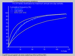
• In hydrology the Pareto distribution is applied to extreme events such as annually maximum one-day rainfalls and river discharges. ^[33] The blue picture illustrates an example of fitting the Pareto distribution to ranked annually maximum one-day rainfalls showing also the 90% confidence belt based on the binomial distribution. The rainfall data are represented by plotting positions as part of the cumulative frequency analysis.
• In Electric Utility Distribution Reliability (80% of the Customer Minutes Interrupted occur on approximately 20% of the days in a given year).

Relation to Zipf's law

The Pareto distribution is a continuous probability distribution. Zipf's law, also sometimes called the zeta distribution, is a discrete distribution, separating the values into a simple ranking. Both are a simple power law with a negative exponent, scaled so that their cumulative distributions equal 1. Zipf's can be derived from the Pareto distribution if the ${\displaystyle x}$ values (incomes) are binned into ${\displaystyle N}$ ranks so that the number of people in each bin follows a 1/rank pattern. The distribution is normalized by defining ${\displaystyle x_{m}}$ so that ${\displaystyle \alpha x_{\mathrm {m} }^{\alpha }={\frac {1}{H(N,\alpha -1)}}}$ where ${\displaystyle H(N,\alpha -1)}$ is the generalized harmonic number. This makes Zipf's probability density function derivable from Pareto's.

${\displaystyle f(x)={\frac {\alpha x_{\mathrm {m} }^{\alpha }}{x^{\alpha +1}}}={\frac {1}{x^{s}H(N,s)}}}$

where ${\displaystyle s=\alpha -1}$ and ${\displaystyle x}$ is an integer representing rank from 1 to N where N is the highest income bracket. So a randomly selected person (or word, website link, or city) from a population (or language, internet, or country) has ${\displaystyle f(x)}$ probability of ranking ${\displaystyle x}$.

Relation to the "Pareto principle"

The "80–20 law", according to which 20% of all people receive 80% of all income, and 20% of the most affluent 20% receive 80% of that 80%, and so on, holds precisely when the Pareto index is ${\displaystyle \alpha =\log _{4}5={\cfrac {\log _{10}5}{\log _{10}4}}\approx 1.161}$. This result can be derived from the Lorenz curve formula given below. Moreover, the following have been shown ^[34] to be mathematically equivalent:

• Income is distributed according to a Pareto distribution with index α > 1.
• There is some number 0 ≤ p ≤ 1/2 such that 100p % of all people receive 100(1 − p)% of all income, and similarly for every real (not necessarily integer) n > 0, 100pⁿ % of all people receive 100(1 − p)ⁿ percentage of all income. α and p are related by

${\displaystyle 1-{\frac {1}{\alpha }}={\frac {\ln(1-p)}{\ln(p)}}={\frac {\ln((1-p)^{n})}{\ln(p^{n})}}}$

This does not apply only to income, but also to wealth, or to anything else that can be modeled by this distribution.

This excludes Pareto distributions in which 0 < α ≤ 1, which, as noted above, have an infinite expected value, and so cannot reasonably model income distribution.

Relation to Price's law

Price's square root law is sometimes offered as a property of or as similar to the Pareto distribution. However, the law only holds in the case that ${\displaystyle \alpha =1}$. Note that in this case, the total and expected amount of wealth are not defined, and the rule only applies asymptotically to random samples. The extended Pareto Principle mentioned above is a far more general rule.

Lorenz curve and Gini coefficient

Lorenz curves for a number of Pareto distributions. The case α = ∞ corresponds to perfectly equal distribution (G = 0) and the α = 1 line corresponds to complete inequality (G = 1)

The Lorenz curve is often used to characterize income and wealth distributions. For any distribution, the Lorenz curve L(F) is written in terms of the PDF f or the CDF F as

${\displaystyle L(F)={\frac {\int _{x_{\mathrm {m} }}^{x(F)}xf(x)\,dx}{\int _{x_{\mathrm {m} }}^{\infty }xf(x)\,dx}}={\frac {\int _{0}^{F}x(F')\,dF'}{\int _{0}^{1}x(F')\,dF'}}}$

where x(F) is the inverse of the CDF. For the Pareto distribution,

${\displaystyle x(F)={\frac {x_{\mathrm {m} }}{(1-F)^{\frac {1}{\alpha }}}}}$

and the Lorenz curve is calculated to be

${\displaystyle L(F)=1-(1-F)^{1-{\frac {1}{\alpha }}},}$

For ${\displaystyle 0<\alpha \leq 1}$ the denominator is infinite, yielding L=0. Examples of the Lorenz curve for a number of Pareto distributions are shown in the graph on the right.

According to Oxfam (2016) the richest 62 people have as much wealth as the poorest half of the world's population. ^[35] We can estimate the Pareto index that would apply to this situation. Letting ε equal ${\displaystyle 62/(7\times 10^{9})}$ we have:

${\displaystyle L(1/2)=1-L(1-\varepsilon )}$

or

${\displaystyle 1-(1/2)^{1-{\frac {1}{\alpha }}}=\varepsilon ^{1-{\frac {1}{\alpha }}}}$

The solution is that α equals about 1.15, and about 9% of the wealth is owned by each of the two groups. But actually the poorest 69% of the world adult population owns only about 3% of the wealth. ^[36]

The Gini coefficient is a measure of the deviation of the Lorenz curve from the equidistribution line which is a line connecting [0, 0] and [1, 1], which is shown in black (α = ∞) in the Lorenz plot on the right. Specifically, the Gini coefficient is twice the area between the Lorenz curve and the equidistribution line. The Gini coefficient for the Pareto distribution is then calculated (for ${\displaystyle \alpha \geq 1}$) to be

${\displaystyle G=1-2\left(\int _{0}^{1}L(F)\,dF\right)={\frac {1}{2\alpha -1}}}$

(see Aaberge 2005).

Random variate generation

Further information: Non-uniform random variate generation

Random samples can be generated using inverse transform sampling. Given a random variate U drawn from the uniform distribution on the unit interval (0, 1], the variate T given by

${\displaystyle T={\frac {x_{\mathrm {m} }}{U^{1/\alpha }}}}$

is Pareto-distributed. ^[37] If U is uniformly distributed on [0, 1), it can be exchanged with (1 − U).

See also

• Bradford's law  – Pattern of references in science journals
• Gutenberg–Richter law  – Law in seismology describing earthquake frequency and magnitude
• Matthew effect  – The rich get richer and the poor get poorer
• Pareto analysis  – Statistical principle about ratio of effects to causesPages displaying short descriptions of redirect targets
• Pareto efficiency  – Optimal allocation of resources
• Pareto interpolation  – Method of estimating the median of a population
• Power law probability distributions  – Functional relationship between two quantities
• Sturgeon's law  – "Ninety percent of everything is crap"
• Traffic generation model  – simulated flow of data in a communications networkPages displaying wikidata descriptions as a fallback
• Zipf's law  – Probability distribution
• Heavy-tailed distribution  – Probability distribution

References

1. Norton, Matthew; Khokhlov, Valentyn; Uryasev, Stan (2019). "Calculating CVaR and bPOE for common probability distributions with application to portfolio optimization and density estimation" (PDF). Annals of Operations Research. Springer. 299 (1–2): 1281–1315. arXiv: 1811.11301 . doi:10.1007/s10479-019-03373-1. S2CID   254231768 . Retrieved 2023-02-27.
2. Amoroso, Luigi (1938). "VILFREDO PARETO". Econometrica (Pre-1986); Jan 1938; 6, 1; ProQuest. 6.
3. Pareto, Vilfredo (1898). "Cours d'economie politique". Journal of Political Economy. 6. doi:10.1086/250536.
4. Pareto, Vilfredo, Cours d'Économie Politique: Nouvelle édition par G.-H. Bousquet et G. Busino, Librairie Droz, Geneva, 1964, pp. 299–345. Original book archived
5. VAN MONTFORT, M.A.J. (1986). "The Generalized Pareto distribution applied to rainfall depths". Hydrological Sciences Journal. 31 (2): 151–162. Bibcode:1986HydSJ..31..151V. doi: 10.1080/02626668609491037 .
6. Oancea, Bogdan (2017). "Income inequality in Romania: The exponential-Pareto distribution". Physica A: Statistical Mechanics and Its Applications. 469: 486–498. Bibcode:2017PhyA..469..486O. doi:10.1016/j.physa.2016.11.094.
7. Morella, Matteo. "Pareto Distribution". academia.edu.
8. Barry C. Arnold (1983). Pareto Distributions. International Co-operative Publishing House. ISBN   978-0-89974-012-6.
9. S. Hussain, S.H. Bhatti (2018). Parameter estimation of Pareto distribution: Some modified moment estimators. Maejo International Journal of Science and Technology 12(1):11-27.
10. Eliazar, Iddo (November 2017). "Lindy's Law". Physica A: Statistical Mechanics and Its Applications. 486: 797–805. Bibcode:2017PhyA..486..797E. doi:10.1016/j.physa.2017.05.077. S2CID   125349686.
11. Johnson NL, Kotz S, Balakrishnan N (1994) Continuous univariate distributions Vol 1. Wiley Series in Probability and Statistics.
12. Johnson, Kotz, and Balakrishnan (1994), (20.4).
13. Christian Kleiber & Samuel Kotz (2003). Statistical Size Distributions in Economics and Actuarial Sciences. Wiley. ISBN   978-0-471-15064-0.
14. Feller, W. (1971). An Introduction to Probability Theory and its Applications. Vol. II (2nd ed.). New York: Wiley. p. 50. "The densities (4.3) are sometimes called after the economist Pareto. It was thought (rather naïvely from a modern statistical standpoint) that income distributions should have a tail with a density ~ Ax^−α as x → ∞".
15. Lomax, K. S. (1954). "Business failures. Another example of the analysis of failure data". Journal of the American Statistical Association. 49 (268): 847–52. doi:10.1080/01621459.1954.10501239.
16. Chotikapanich, Duangkamon (16 September 2008). "Chapter 7: Pareto and Generalized Pareto Distributions". Modeling Income Distributions and Lorenz Curves. Springer. pp. 121–22. ISBN   9780387727967.
17. Dallas, A. C. "Characterizing the Pareto and power distributions." Annals of the Institute of Statistical Mathematics 28.1 (1976): 491-497.
18. White, Gentry (2006). Bayesian semiparametric spatial and joint spatio-temporal modeling (Thesis thesis). University of Missouri--Columbia. section 5.3.1.
19. "Inverse Transform Method". Archived from the original on 2012-01-17. Retrieved 2012-08-27.
20. Huang, Xiao-dong (2004). "A Multiscale Model for MPEG-4 Varied Bit Rate Video Traffic". IEEE Transactions on Broadcasting. 50 (3): 323–334. doi:10.1109/TBC.2004.834013.
21. Rootzén, Holger; Tajvidi, Nader (2006). "Multivariate generalized Pareto distributions". Bernoulli. 12 (5): 917–30. CiteSeerX   10.1.1.145.2991 . doi:10.3150/bj/1161614952. S2CID   16504396.
22. M. E. J. Newman (2005). "Power laws, Pareto distributions and Zipf's law". Contemporary Physics . 46 (5): 323–51. arXiv: cond-mat/0412004 . Bibcode:2005ConPh..46..323N. doi:10.1080/00107510500052444. S2CID   202719165.
23. H. J. Malik (1970). "Estimation of the Parameters of the Pareto Distribution". Metrika. 15: 126–132. doi:10.1007/BF02613565. S2CID   124007966.
24. For a two-quantile population, where approximately 18% of the population owns 82% of the wealth, the Theil index takes the value 1.
25. Gaillard, Alexandre; Hellwig, Christian; Wangner, Philipp; Werquin, Nicolas (2023). "Consumption, Wealth, and Income Inequality: A Tale of Tails". SSRN   4636704.
26. Reed, William J.; et al. (2004). "The Double Pareto-Lognormal Distribution – A New Parametric Model for Size Distributions". Communications in Statistics – Theory and Methods. 33 (8): 1733–53. CiteSeerX   10.1.1.70.4555 . doi:10.1081/sta-120037438. S2CID   13906086.
27. Reed, William J. (2002). "On the rank-size distribution for human settlements". Journal of Regional Science. 42 (1): 1–17. Bibcode:2002JRegS..42....1R. doi:10.1111/1467-9787.00247. S2CID   154285730.
28. Schroeder, Bianca; Damouras, Sotirios; Gill, Phillipa (2010-02-24). "Understanding latent sector error and how to protect against them" (PDF). 8th Usenix Conference on File and Storage Technologies (FAST 2010). Retrieved 2010-09-10. We experimented with 5 different distributions (Geometric, Weibull, Rayleigh, Pareto, and Lognormal), that are commonly used in the context of system reliability, and evaluated their fit through the total squared differences between the actual and hypothesized frequencies (χ² statistic). We found consistently across all models that the geometric distribution is a poor fit, while the Pareto distribution provides the best fit.
29. Yuji Ijiri; Simon, Herbert A. (May 1975). "Some Distributions Associated with Bose–Einstein Statistics". Proc. Natl. Acad. Sci. USA. 72 (5): 1654–57. Bibcode:1975PNAS...72.1654I. doi: 10.1073/pnas.72.5.1654 . PMC   432601 . PMID   16578724.
30. Harchol-Balter, Mor; Downey, Allen (August 1997). "Exploiting Process Lifetime Distributions for Dynamic Load Balancing" (PDF). ACM Transactions on Computer Systems. 15 (3): 253–258. doi:10.1145/263326.263344. S2CID   52861447.
31. Kleiber and Kotz (2003): p. 94.
32. Seal, H. (1980). "Survival probabilities based on Pareto claim distributions". ASTIN Bulletin. 11: 61–71. doi: 10.1017/S0515036100006620 .
33. CumFreq, software for cumulative frequency analysis and probability distribution fitting
34. Hardy, Michael (2010). "Pareto's Law". Mathematical Intelligencer . 32 (3): 38–43. doi:10.1007/s00283-010-9159-2. S2CID   121797873.
35. "62 people own the same as half the world, reveals Oxfam Davos report". Oxfam. Jan 2016.
36. "Global Wealth Report 2013". Credit Suisse. Oct 2013. p. 22. Archived from the original on 2015-02-14. Retrieved 2016-01-24.
37. Tanizaki, Hisashi (2004). Computational Methods in Statistics and Econometrics. CRC Press. p. 133. ISBN   9780824750886.

Notes

• M. O. Lorenz (1905). "Methods of measuring the concentration of wealth". Publications of the American Statistical Association . 9 (70): 209–19. Bibcode:1905PAmSA...9..209L. doi:10.2307/2276207. JSTOR   2276207. S2CID   154048722.
• Pareto, Vilfredo (1965). Librairie Droz (ed.). Ecrits sur la courbe de la répartition de la richesse. Œuvres complètes : T. III. p. 48. ISBN   9782600040211.

• Pareto, Vilfredo (1895). "La legge della domanda". Giornale Degli Economisti. 10: 59–68.
• Pareto, Vilfredo (1896). "Cours d'économie politique". doi:10.1177/000271629700900314. S2CID   143528002.{{cite journal}}: Cite journal requires |journal= (help)

External links

• "Pareto distribution", Encyclopedia of Mathematics , EMS Press, 2001 [1994]
• Weisstein, Eric W. "Pareto distribution". MathWorld .
• Aabergé, Rolf (May 2005). "Gini's Nuclear Family". International Conference to Honor Two Eminent Social Scientists (PDF).

• Crovella, Mark E.; Bestavros, Azer (December 1997). Self-Similarity in World Wide Web Traffic: Evidence and Possible Causes (PDF). IEEE/ACM Transactions on Networking. Vol. 5. pp. 835–846. Archived from the original (PDF) on 2016-03-04. Retrieved 2019-02-25.

• syntraf1.c is a C program to generate synthetic packet traffic with bounded Pareto burst size and exponential interburst time.