Normal-inverse-gamma distribution

normal-inverse-gamma

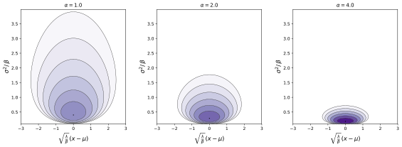
Probability density function
Parameters	${\displaystyle \mu \,}$ location (real) ${\displaystyle \lambda >0\,}$ (real) ${\displaystyle \alpha >0\,}$ (real) ${\displaystyle \beta >0\,}$ (real)
Support	${\displaystyle x\in (-\infty ,\infty )\,\!,\;\sigma ^{2}\in (0,\infty )}$
PDF	${\displaystyle {\frac {\sqrt {\lambda }}{\sqrt {2\pi \sigma ^{2}}}}{\frac {\beta ^{\alpha }}{\Gamma (\alpha )}}\left({\frac {1}{\sigma ^{2}}}\right)^{\alpha +1}\exp \left(-{\frac {2\beta +\lambda (x-\mu )^{2}}{2\sigma ^{2}}}\right)}$
Mean	${\displaystyle \operatorname {E} [x]=\mu }$ ${\displaystyle \operatorname {E} [\sigma ^{2}]={\frac {\beta }{\alpha -1}}}$, for ${\displaystyle \alpha >1}$
Mode	${\displaystyle x=\mu \;{\textrm {(univariate)}},x={\boldsymbol {\mu }}\;{\textrm {(multivariate)}}}$ ${\displaystyle \sigma ^{2}={\frac {\beta }{\alpha +1+1/2}}\;{\textrm {(univariate)}},\sigma ^{2}={\frac {\beta }{\alpha +1+k/2}}\;{\textrm {(multivariate)}}}$
Variance	${\displaystyle \operatorname {Var} [x]={\frac {\beta }{(\alpha -1)\lambda }}}$, for ${\displaystyle \alpha >1}$ ${\displaystyle \operatorname {Var} [\sigma ^{2}]={\frac {\beta ^{2}}{(\alpha -1)^{2}(\alpha -2)}}}$, for ${\displaystyle \alpha >2}$ ${\displaystyle \operatorname {Cov} [x,\sigma ^{2}]=0}$, for ${\displaystyle \alpha >1}$

In probability theory and statistics, the normal-inverse-gamma distribution (or Gaussian-inverse-gamma distribution) is a four-parameter family of multivariate continuous probability distributions. It is the conjugate prior of a normal distribution with unknown mean and variance.

Definition

Suppose

${\displaystyle x\mid \sigma ^{2},\mu ,\lambda \sim \mathrm {N} (\mu ,\sigma ^{2}/\lambda )\,\!}$

has a normal distribution with mean ${\displaystyle \mu }$ and variance ${\displaystyle \sigma ^{2}/\lambda }$, where

${\displaystyle \sigma ^{2}\mid \alpha ,\beta \sim \Gamma ^{-1}(\alpha ,\beta )\!}$

has an inverse-gamma distribution. Then ${\displaystyle (x,\sigma ^{2})}$ has a normal-inverse-gamma distribution, denoted as

${\displaystyle (x,\sigma ^{2})\sim {\text{N-}}\Gamma ^{-1}(\mu ,\lambda ,\alpha ,\beta )\!.}$

(${\displaystyle {\text{NIG}}}$ is also used instead of ${\displaystyle {\text{N-}}\Gamma ^{-1}.}$)

The normal-inverse-Wishart distribution is a generalization of the normal-inverse-gamma distribution that is defined over multivariate random variables.

Characterization

Probability density function

${\displaystyle f(x,\sigma ^{2}\mid \mu ,\lambda ,\alpha ,\beta )={\frac {\sqrt {\lambda }}{\sigma {\sqrt {2\pi }}}}\,{\frac {\beta ^{\alpha }}{\Gamma (\alpha )}}\,\left({\frac {1}{\sigma ^{2}}}\right)^{\alpha +1}\exp \left(-{\frac {2\beta +\lambda (x-\mu )^{2}}{2\sigma ^{2}}}\right)}$

For the multivariate form where ${\displaystyle \mathbf {x} }$ is a ${\displaystyle k\times 1}$ random vector,

${\displaystyle f(\mathbf {x} ,\sigma ^{2}\mid \mu ,\mathbf {V} ^{-1},\alpha ,\beta )=|\mathbf {V} |^{-1/2}{(2\pi )^{-k/2}}\,{\frac {\beta ^{\alpha }}{\Gamma (\alpha )}}\,\left({\frac {1}{\sigma ^{2}}}\right)^{\alpha +1+k/2}\exp \left(-{\frac {2\beta +(\mathbf {x} -{\boldsymbol {\mu }})^{T}\mathbf {V} ^{-1}(\mathbf {x} -{\boldsymbol {\mu }})}{2\sigma ^{2}}}\right).}$

where ${\displaystyle |\mathbf {V} |}$ is the determinant of the ${\displaystyle k\times k}$ matrix ${\displaystyle \mathbf {V} }$. Note how this last equation reduces to the first form if ${\displaystyle k=1}$ so that ${\displaystyle \mathbf {x} ,\mathbf {V} ,{\boldsymbol {\mu }}}$ are scalars.

Alternative parameterization

It is also possible to let ${\displaystyle \gamma =1/\lambda }$ in which case the pdf becomes

${\displaystyle f(x,\sigma ^{2}\mid \mu ,\gamma ,\alpha ,\beta )={\frac {1}{\sigma {\sqrt {2\pi \gamma }}}}\,{\frac {\beta ^{\alpha }}{\Gamma (\alpha )}}\,\left({\frac {1}{\sigma ^{2}}}\right)^{\alpha +1}\exp \left(-{\frac {2\gamma \beta +(x-\mu )^{2}}{2\gamma \sigma ^{2}}}\right)}$

In the multivariate form, the corresponding change would be to regard the covariance matrix ${\displaystyle \mathbf {V} }$ instead of its inverse ${\displaystyle \mathbf {V} ^{-1}}$ as a parameter.

Cumulative distribution function

${\displaystyle F(x,\sigma ^{2}\mid \mu ,\lambda ,\alpha ,\beta )={\frac {e^{-{\frac {\beta }{\sigma ^{2}}}}\left({\frac {\beta }{\sigma ^{2}}}\right)^{\alpha }\left(\operatorname {erf} \left({\frac {{\sqrt {\lambda }}(x-\mu )}{{\sqrt {2}}\sigma }}\right)+1\right)}{2\sigma ^{2}\Gamma (\alpha )}}}$

Properties

Marginal distributions

Given ${\displaystyle (x,\sigma ^{2})\sim {\text{N-}}\Gamma ^{-1}(\mu ,\lambda ,\alpha ,\beta )\!.}$ as above, ${\displaystyle \sigma ^{2}}$ by itself follows an inverse gamma distribution:

${\displaystyle \sigma ^{2}\sim \Gamma ^{-1}(\alpha ,\beta )\!}$

while ${\displaystyle {\sqrt {\frac {\alpha \lambda }{\beta }}}(x-\mu )}$ follows a t distribution with ${\displaystyle 2\alpha }$ degrees of freedom. ^[1]

Proof for ${\displaystyle \lambda =1}$

For ${\displaystyle \lambda =1}$ probability density function is

${\displaystyle f(x,\sigma ^{2}\mid \mu ,\alpha ,\beta )={\frac {1}{\sigma {\sqrt {2\pi }}}}\,{\frac {\beta ^{\alpha }}{\Gamma (\alpha )}}\,\left({\frac {1}{\sigma ^{2}}}\right)^{\alpha +1}\exp \left(-{\frac {2\beta +(x-\mu )^{2}}{2\sigma ^{2}}}\right)}$

Marginal distribution over ${\displaystyle x}$ is

${\displaystyle {\begin{aligned}f(x\mid \mu ,\alpha ,\beta )&=\int _{0}^{\infty }d\sigma ^{2}f(x,\sigma ^{2}\mid \mu ,\alpha ,\beta )\\&={\frac {1}{\sqrt {2\pi }}}\,{\frac {\beta ^{\alpha }}{\Gamma (\alpha )}}\int _{0}^{\infty }d\sigma ^{2}\left({\frac {1}{\sigma ^{2}}}\right)^{\alpha +1/2+1}\exp \left(-{\frac {2\beta +(x-\mu )^{2}}{2\sigma ^{2}}}\right)\end{aligned}}}$

Except for normalization factor, expression under the integral coincides with Inverse-gamma distribution

${\displaystyle \Gamma ^{-1}(x;a,b)={\frac {b^{a}}{\Gamma (a)}}{\frac {e^{-b/x}}{{x}^{a+1}}},}$

with ${\displaystyle x=\sigma ^{2}}$, ${\displaystyle a=\alpha +1/2}$, ${\displaystyle b={\frac {2\beta +(x-\mu )^{2}}{2}}}$.

Since ${\displaystyle \int _{0}^{\infty }dx\Gamma ^{-1}(x;a,b)=1,\quad \int _{0}^{\infty }dxx^{-(a+1)}e^{-b/x}=\Gamma (a)b^{-a}}$, and

${\displaystyle \int _{0}^{\infty }d\sigma ^{2}\left({\frac {1}{\sigma ^{2}}}\right)^{\alpha +1/2+1}\exp \left(-{\frac {2\beta +(x-\mu )^{2}}{2\sigma ^{2}}}\right)=\Gamma (\alpha +1/2)\left({\frac {2\beta +(x-\mu )^{2}}{2}}\right)^{-(\alpha +1/2)}}$

Substituting this expression and factoring dependence on ${\displaystyle x}$,

${\displaystyle f(x\mid \mu ,\alpha ,\beta )\propto _{x}\left(1+{\frac {(x-\mu )^{2}}{2\beta }}\right)^{-(\alpha +1/2)}.}$

Shape of generalized Student's t-distribution is

${\displaystyle t(x|\nu ,{\hat {\mu }},{\hat {\sigma }}^{2})\propto _{x}\left(1+{\frac {1}{\nu }}{\frac {(x-{\hat {\mu }})^{2}}{{\hat {\sigma }}^{2}}}\right)^{-(\nu +1)/2}}$.

Marginal distribution ${\displaystyle f(x\mid \mu ,\alpha ,\beta )}$ follows t-distribution with ${\displaystyle 2\alpha }$ degrees of freedom

${\displaystyle f(x\mid \mu ,\alpha ,\beta )=t(x|\nu =2\alpha ,{\hat {\mu }}=\mu ,{\hat {\sigma }}^{2}=\beta /\alpha )}$.

In the multivariate case, the marginal distribution of ${\displaystyle \mathbf {x} }$ is a multivariate t distribution:

${\displaystyle \mathbf {x} \sim t_{2\alpha }({\boldsymbol {\mu }},{\frac {\beta }{\alpha }}\mathbf {V} )\!}$

Scaling

Suppose

${\displaystyle (x,\sigma ^{2})\sim {\text{N-}}\Gamma ^{-1}(\mu ,\lambda ,\alpha ,\beta )\!.}$

Then for ${\displaystyle c>0}$,

${\displaystyle (cx,c\sigma ^{2})\sim {\text{N-}}\Gamma ^{-1}(c\mu ,\lambda /c,\alpha ,c\beta )\!.}$

Proof: To prove this let ${\displaystyle (x,\sigma ^{2})\sim {\text{N-}}\Gamma ^{-1}(\mu ,\lambda ,\alpha ,\beta )}$ and fix ${\displaystyle c>0}$. Defining ${\displaystyle Y=(Y_{1},Y_{2})=(cx,c\sigma ^{2})}$, observe that the PDF of the random variable ${\displaystyle Y}$ evaluated at ${\displaystyle (y_{1},y_{2})}$ is given by ${\displaystyle 1/c^{2}}$ times the PDF of a ${\displaystyle {\text{N-}}\Gamma ^{-1}(\mu ,\lambda ,\alpha ,\beta )}$ random variable evaluated at ${\displaystyle (y_{1}/c,y_{2}/c)}$. Hence the PDF of ${\displaystyle Y}$ evaluated at ${\displaystyle (y_{1},y_{2})}$ is given by :${\displaystyle f_{Y}(y_{1},y_{2})={\frac {1}{c^{2}}}{\frac {\sqrt {\lambda }}{\sqrt {2\pi y_{2}/c}}}\,{\frac {\beta ^{\alpha }}{\Gamma (\alpha )}}\,\left({\frac {1}{y_{2}/c}}\right)^{\alpha +1}\exp \left(-{\frac {2\beta +\lambda (y_{1}/c-\mu )^{2}}{2y_{2}/c}}\right)={\frac {\sqrt {\lambda /c}}{\sqrt {2\pi y_{2}}}}\,{\frac {(c\beta )^{\alpha }}{\Gamma (\alpha )}}\,\left({\frac {1}{y_{2}}}\right)^{\alpha +1}\exp \left(-{\frac {2c\beta +(\lambda /c)\,(y_{1}-c\mu )^{2}}{2y_{2}}}\right).\!}$

The right hand expression is the PDF for a ${\displaystyle {\text{N-}}\Gamma ^{-1}(c\mu ,\lambda /c,\alpha ,c\beta )}$ random variable evaluated at ${\displaystyle (y_{1},y_{2})}$, which completes the proof.

Exponential family

Normal-inverse-gamma distributions form an exponential family with natural parameters ${\displaystyle \textstyle \theta _{1}={\frac {-\lambda }{2}}}$, ${\displaystyle \textstyle \theta _{2}=\lambda \mu }$, ${\displaystyle \textstyle \theta _{3}=\alpha }$, and ${\displaystyle \textstyle \theta _{4}=-\beta +{\frac {-\lambda \mu ^{2}}{2}}}$ and sufficient statistics ${\displaystyle \textstyle T_{1}={\frac {x^{2}}{\sigma ^{2}}}}$, ${\displaystyle \textstyle T_{2}={\frac {x}{\sigma ^{2}}}}$, ${\displaystyle \textstyle T_{3}=\log {\big (}{\frac {1}{\sigma ^{2}}}{\big )}}$, and ${\displaystyle \textstyle T_{4}={\frac {1}{\sigma ^{2}}}}$.

Kullback–Leibler divergence

Measures difference between two distributions.

Posterior distribution of the parameters

See the articles on normal-gamma distribution and conjugate prior.

Interpretation of the parameters

See the articles on normal-gamma distribution and conjugate prior.

Generating normal-inverse-gamma random variates

Generation of random variates is straightforward:

1. Sample ${\displaystyle \sigma ^{2}}$ from an inverse gamma distribution with parameters ${\displaystyle \alpha }$ and ${\displaystyle \beta }$
2. Sample ${\displaystyle x}$ from a normal distribution with mean ${\displaystyle \mu }$ and variance ${\displaystyle \sigma ^{2}/\lambda }$

Related distributions

• The normal-gamma distribution is the same distribution parameterized by precision rather than variance
• A generalization of this distribution which allows for a multivariate mean and a completely unknown positive-definite covariance matrix ${\displaystyle \sigma ^{2}\mathbf {V} }$ (whereas in the multivariate inverse-gamma distribution the covariance matrix is regarded as known up to the scale factor ${\displaystyle \sigma ^{2}}$) is the normal-inverse-Wishart distribution

See also

• Compound probability distribution

References

1. Ramírez-Hassan, Andrés. 4.2 Conjugate prior to exponential family | Introduction to Bayesian Econometrics.

• Denison, David G. T.; Holmes, Christopher C.; Mallick, Bani K.; Smith, Adrian F. M. (2002) Bayesian Methods for Nonlinear Classification and Regression, Wiley. ISBN   0471490369
• Koch, Karl-Rudolf (2007) Introduction to Bayesian Statistics (2nd Edition), Springer. ISBN   354072723X