
The Cauchy distribution, named after Augustin Cauchy, is a continuous probability distribution. It is also known, especially among physicists, as the Lorentz distribution, Cauchy–Lorentz distribution, Lorentz(ian) function, or Breit–Wigner distribution. The Cauchy distribution is the distribution of the x-intercept of a ray issuing from with a uniformly distributed angle. It is also the distribution of the ratio of two independent normally distributed random variables with mean zero.

The Pareto distribution, named after the Italian civil engineer, economist, and sociologist Vilfredo Pareto, is a power-law probability distribution that is used in description of social, quality control, scientific, geophysical, actuarial, and many other types of observable phenomena; the principle originally applied to describing the distribution of wealth in a society, fitting the trend that a large portion of wealth is held by a small fraction of the population. The Pareto principle or "80-20 rule" stating that 80% of outcomes are due to 20% of causes was named in honour of Pareto, but the concepts are distinct, and only Pareto distributions with shape value of log45 ≈ 1.16 precisely reflect it. Empirical observation has shown that this 80-20 distribution fits a wide range of cases, including natural phenomena and human activities.
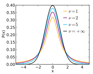
In probability and statistics, Student's t distribution is a continuous probability distribution that generalizes the standard normal distribution. Like the latter, it is symmetric around zero and bell-shaped.

In probability theory and statistics, the Weibull distribution is a continuous probability distribution. It models a broad range of random variables, largely in the nature of a time to failure or time between events. Examples are maximum one-day rainfalls and the time a user spends on a web page.

In probability theory and statistics, the beta distribution is a family of continuous probability distributions defined on the interval [0, 1] or in terms of two positive parameters, denoted by alpha (α) and beta (β), that appear as exponents of the variable and its complement to 1, respectively, and control the shape of the distribution.

In probability theory and statistics, the Gumbel distribution is used to model the distribution of the maximum of a number of samples of various distributions.

In probability theory, a distribution is said to be stable if a linear combination of two independent random variables with this distribution has the same distribution, up to location and scale parameters. A random variable is said to be stable if its distribution is stable. The stable distribution family is also sometimes referred to as the Lévy alpha-stable distribution, after Paul Lévy, the first mathematician to have studied it.
In probability theory and statistics, the generalized extreme value (GEV) distribution is a family of continuous probability distributions developed within extreme value theory to combine the Gumbel, Fréchet and Weibull families also known as type I, II and III extreme value distributions. By the extreme value theorem the GEV distribution is the only possible limit distribution of properly normalized maxima of a sequence of independent and identically distributed random variables. Note that a limit distribution needs to exist, which requires regularity conditions on the tail of the distribution. Despite this, the GEV distribution is often used as an approximation to model the maxima of long (finite) sequences of random variables.
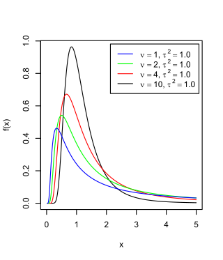
The scaled inverse chi-squared distribution is the distribution for x = 1/s2, where s2 is a sample mean of the squares of ν independent normal random variables that have mean 0 and inverse variance 1/σ2 = τ2. The distribution is therefore parametrised by the two quantities ν and τ2, referred to as the number of chi-squared degrees of freedom and the scaling parameter, respectively.

In probability theory and directional statistics, the von Mises distribution is a continuous probability distribution on the circle. It is a close approximation to the wrapped normal distribution, which is the circular analogue of the normal distribution. A freely diffusing angle on a circle is a wrapped normally distributed random variable with an unwrapped variance that grows linearly in time. On the other hand, the von Mises distribution is the stationary distribution of a drift and diffusion process on the circle in a harmonic potential, i.e. with a preferred orientation. The von Mises distribution is the maximum entropy distribution for circular data when the real and imaginary parts of the first circular moment are specified. The von Mises distribution is a special case of the von Mises–Fisher distribution on the N-dimensional sphere.
The noncentral t-distribution generalizes Student's t-distribution using a noncentrality parameter. Whereas the central probability distribution describes how a test statistic t is distributed when the difference tested is null, the noncentral distribution describes how t is distributed when the null is false. This leads to its use in statistics, especially calculating statistical power. The noncentral t-distribution is also known as the singly noncentral t-distribution, and in addition to its primary use in statistical inference, is also used in robust modeling for data.
The cross-entropy (CE) method is a Monte Carlo method for importance sampling and optimization. It is applicable to both combinatorial and continuous problems, with either a static or noisy objective.

In probability and statistics, the truncated normal distribution is the probability distribution derived from that of a normally distributed random variable by bounding the random variable from either below or above. The truncated normal distribution has wide applications in statistics and econometrics.
The Birnbaum–Saunders distribution, also known as the fatigue life distribution, is a probability distribution used extensively in reliability applications to model failure times. There are several alternative formulations of this distribution in the literature. It is named after Z. W. Birnbaum and S. C. Saunders.

The shifted log-logistic distribution is a probability distribution also known as the generalized log-logistic or the three-parameter log-logistic distribution. It has also been called the generalized logistic distribution, but this conflicts with other uses of the term: see generalized logistic distribution.

In probability theory and statistics, the skew normal distribution is a continuous probability distribution that generalises the normal distribution to allow for non-zero skewness.
The generalized normal distribution or generalized Gaussian distribution (GGD) is either of two families of parametric continuous probability distributions on the real line. Both families add a shape parameter to the normal distribution. To distinguish the two families, they are referred to below as "symmetric" and "asymmetric"; however, this is not a standard nomenclature.
In probability and statistics, the generalized K-distribution is a three-parameter family of continuous probability distributions. The distribution arises by compounding two gamma distributions. In each case, a re-parametrization of the usual form of the family of gamma distributions is used, such that the parameters are:

The Lomax distribution, conditionally also called the Pareto Type II distribution, is a heavy-tail probability distribution used in business, economics, actuarial science, queueing theory and Internet traffic modeling. It is named after K. S. Lomax. It is essentially a Pareto distribution that has been shifted so that its support begins at zero.
In probability theory and statistics, an inverse distribution is the distribution of the reciprocal of a random variable. Inverse distributions arise in particular in the Bayesian context of prior distributions and posterior distributions for scale parameters. In the algebra of random variables, inverse distributions are special cases of the class of ratio distributions, in which the numerator random variable has a degenerate distribution.


