Gamma distribution

Gamma

Probability density function
Cumulative distribution function
Parameters	k > 0 shape θ > 0 scale	α > 0 shape β > 0 rate
Support	${\displaystyle x\in (0,\infty )}$	${\displaystyle x\in (0,\infty )}$
PDF	${\displaystyle f(x)={\frac {1}{\Gamma (k)\theta ^{k}}}x^{k-1}e^{-x/\theta }}$	${\displaystyle f(x)={\frac {\beta ^{\alpha }}{\Gamma (\alpha )}}x^{\alpha -1}e^{-\beta x}}$
CDF	${\displaystyle F(x)={\frac {1}{\Gamma (k)}}\gamma \left(k,{\frac {x}{\theta }}\right)}$	${\displaystyle F(x)={\frac {1}{\Gamma (\alpha )}}\gamma (\alpha ,\beta x)}$
Mean	${\displaystyle k\theta }$	${\displaystyle {\frac {\alpha }{\beta }}}$
Median	No simple closed form	No simple closed form
Mode	${\displaystyle (k-1)\theta {\text{ for }}k\geq 1}$, ${\displaystyle 0{\text{ for }}k<1}$	${\displaystyle {\frac {\alpha -1}{\beta }}{\text{ for }}\alpha \geq 1{\text{, }}0{\text{ for }}\alpha <1}$
Variance	${\displaystyle k\theta ^{2}}$	${\displaystyle {\frac {\alpha }{\beta ^{2}}}}$
Skewness	${\displaystyle {\frac {2}{\sqrt {k}}}}$	${\displaystyle {\frac {2}{\sqrt {\alpha }}}}$
Excess kurtosis	${\displaystyle {\frac {6}{k}}}$	${\displaystyle {\frac {6}{\alpha }}}$
Entropy	${\displaystyle {\begin{aligned}k&+\ln \theta +\ln \Gamma (k)\\&+(1-k)\psi (k)\end{aligned}}}$	${\displaystyle {\begin{aligned}\alpha &-\ln \beta +\ln \Gamma (\alpha )\\&+(1-\alpha )\psi (\alpha )\end{aligned}}}$
MGF	${\displaystyle (1-\theta t)^{-k}{\text{ for }}t<{\frac {1}{\theta }}}$	${\displaystyle \left(1-{\frac {t}{\beta }}\right)^{-\alpha }{\text{ for }}t<\beta }$
CF	${\displaystyle (1-\theta it)^{-k}}$	${\displaystyle \left(1-{\frac {it}{\beta }}\right)^{-\alpha }}$
Fisher information	${\displaystyle I(k,\theta )={\begin{pmatrix}\psi ^{(1)}(k)&\theta ^{-1}\\\theta ^{-1}&k\theta ^{-2}\end{pmatrix}}}$	${\displaystyle I(\alpha ,\beta )={\begin{pmatrix}\psi ^{(1)}(\alpha )&-\beta ^{-1}\\-\beta ^{-1}&\alpha \beta ^{-2}\end{pmatrix}}}$
Method of Moments	${\displaystyle k={\frac {E[X]^{2}}{V[X]}}\quad \quad }$${\displaystyle \theta ={\frac {V[X]}{E[X]}}\quad \quad }$	${\displaystyle \alpha ={\frac {E[X]^{2}}{V[X]}}}$${\displaystyle \beta ={\frac {E[X]}{V[X]}}}$

In probability theory and statistics, the gamma distribution is a versatile two-parameter family of continuous probability distributions. The exponential distribution, Erlang distribution, and chi-squared distribution are special cases of the gamma distribution. There are two equivalent parameterizations in common use:

1. With a shape parameter k and a scale parameter θ
2. With a shape parameter ${\displaystyle \alpha =k}$ and an inverse scale parameter ${\displaystyle \beta =1/\theta }$ , called a rate parameter.

In each of these forms, both parameters are positive real numbers.

The distribution has significant applications across various fields, including econometrics, Bayesian statistics, life testing. In econometrics, the (k, θ) parameterization is common for modeling waiting times, such as the time until death, where it often takes the form of an Erlang distribution for integer k values. Bayesian statistics prefer the (α, β) parameterization, utilizing the gamma distribution as a conjugate prior for several inverse scale parameters, facilitating analytical tractability in posterior distribution computations. The probability density and cumulative distribution functions of the gamma distribution vary based on the chosen parameterization, both offering insights into the behavior of gamma-distributed random variables. The gamma distribution is integral to modeling a range of phenomena due to its flexible shape, which can capture various statistical distributions, including the exponential and chi-squared distributions under specific conditions. Its mathematical properties, such as mean, variance, skewness, and higher moments, provide a toolset for statistical analysis and inference. Practical applications of the distribution span several disciplines, underscoring its importance in theoretical and applied statistics.

The gamma distribution is the maximum entropy probability distribution (both with respect to a uniform base measure and a ${\displaystyle 1/x}$ base measure) for a random variable X for which E[X] = kθ = α/β is fixed and greater than zero, and E[ln X] = ψ(k) + ln θ = ψ(α) − ln β is fixed (ψ is the digamma function). ^[1]

Definitions

The parameterization with k and θ appears to be more common in econometrics and other applied fields, where the gamma distribution is frequently used to model waiting times. For instance, in life testing, the waiting time until death is a random variable that is frequently modeled with a gamma distribution. See Hogg and Craig ^[2] for an explicit motivation.

The parameterization with α and β is more common in Bayesian statistics, where the gamma distribution is used as a conjugate prior distribution for various types of inverse scale (rate) parameters, such as the λ of an exponential distribution or a Poisson distribution ^[3] – or for that matter, the β of the gamma distribution itself. The closely related inverse-gamma distribution is used as a conjugate prior for scale parameters, such as the variance of a normal distribution.

If k is a positive integer, then the distribution represents an Erlang distribution; i.e., the sum of k independent exponentially distributed random variables, each of which has a mean of θ.

Characterization using shape α and rate β

The gamma distribution can be parameterized in terms of a shape parameter α = k and an inverse scale parameter β = 1/θ, called a rate parameter. A random variable X that is gamma-distributed with shape α and rate β is denoted

${\displaystyle X\sim \Gamma (\alpha ,\beta )\equiv \operatorname {Gamma} (\alpha ,\beta )}$

The corresponding probability density function in the shape-rate parameterization is

${\displaystyle {\begin{aligned}f(x;\alpha ,\beta )&={\frac {x^{\alpha -1}e^{-\beta x}\beta ^{\alpha }}{\Gamma (\alpha )}}\quad {\text{ for }}x>0\quad \alpha ,\beta >0,\\[6pt]\end{aligned}}}$

where ${\displaystyle \Gamma (\alpha )}$ is the gamma function. For all positive integers, ${\displaystyle \Gamma (\alpha )=(\alpha -1)!}$.

The cumulative distribution function is the regularized gamma function:

${\displaystyle F(x;\alpha ,\beta )=\int _{0}^{x}f(u;\alpha ,\beta )\,du={\frac {\gamma (\alpha ,\beta x)}{\Gamma (\alpha )}},}$

where ${\displaystyle \gamma (\alpha ,\beta x)}$ is the lower incomplete gamma function.

If α is a positive integer (i.e., the distribution is an Erlang distribution), the cumulative distribution function has the following series expansion: ^[4]

${\displaystyle F(x;\alpha ,\beta )=1-\sum _{i=0}^{\alpha -1}{\frac {(\beta x)^{i}}{i!}}e^{-\beta x}=e^{-\beta x}\sum _{i=\alpha }^{\infty }{\frac {(\beta x)^{i}}{i!}}.}$

Characterization using shape k and scale θ

A random variable X that is gamma-distributed with shape k and scale θ is denoted by

${\displaystyle X\sim \Gamma (k,\theta )\equiv \operatorname {Gamma} (k,\theta )}$

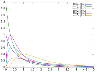
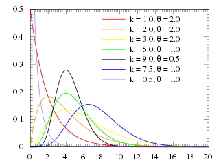
Illustration of the gamma PDF for parameter values over k and x with θ set to 1, 2, 3, 4, 5, and 6. One can see each θ layer by itself here as well as by k and x. .

The probability density function using the shape-scale parametrization is

${\displaystyle f(x;k,\theta )={\frac {x^{k-1}e^{-x/\theta }}{\theta ^{k}\Gamma (k)}}\quad {\text{ for }}x>0{\text{ and }}k,\theta >0.}$

Here Γ(k) is the gamma function evaluated at k.

The cumulative distribution function is the regularized gamma function:

${\displaystyle F(x;k,\theta )=\int _{0}^{x}f(u;k,\theta )\,du={\frac {\gamma \left(k,{\frac {x}{\theta }}\right)}{\Gamma (k)}},}$

where ${\displaystyle \gamma \left(k,{\frac {x}{\theta }}\right)}$ is the lower incomplete gamma function.

It can also be expressed as follows, if k is a positive integer (i.e., the distribution is an Erlang distribution): ^[4]

${\displaystyle F(x;k,\theta )=1-\sum _{i=0}^{k-1}{\frac {1}{i!}}\left({\frac {x}{\theta }}\right)^{i}e^{-x/\theta }=e^{-x/\theta }\sum _{i=k}^{\infty }{\frac {1}{i!}}\left({\frac {x}{\theta }}\right)^{i}.}$

Both parametrizations are common because either can be more convenient depending on the situation.

Properties

Mean and variance

The mean of gamma distribution is given by the product of its shape and scale parameters:

${\displaystyle \mu =k\theta =\alpha /\beta }$

The variance is:

${\displaystyle \sigma ^{2}=k\theta ^{2}=\alpha /\beta ^{2}}$

The square root of the inverse shape parameter gives the coefficient of variation:

${\displaystyle \sigma /\mu =k^{-0.5}=1/{\sqrt {\alpha }}}$

Skewness

The skewness of the gamma distribution only depends on its shape parameter, k, and it is equal to ${\displaystyle 2/{\sqrt {k}}.}$

Higher moments

The n-th raw moment is given by:

${\displaystyle \mathrm {E} [X^{n}]=\theta ^{n}{\frac {\Gamma (k+n)}{\Gamma (k)}}=\theta ^{n}\prod _{i=1}^{n}(k+i-1)\;{\text{ for }}n=1,2,\ldots .}$

Median approximations and bounds

Bounds and asymptotic approximations to the median of the gamma distribution. The cyan-colored region indicates the large gap between published lower and upper bounds.

Unlike the mode and the mean, which have readily calculable formulas based on the parameters, the median does not have a closed-form equation. The median for this distribution is the value ν such that

${\displaystyle {\frac {1}{\Gamma (k)\theta ^{k}}}\int _{0}^{\nu }x^{k-1}e^{-x/\theta }dx={\frac {1}{2}}.}$

A rigorous treatment of the problem of determining an asymptotic expansion and bounds for the median of the gamma distribution was handled first by Chen and Rubin, who proved that (for ${\displaystyle \theta =1}$)

${\displaystyle k-{\frac {1}{3}}<\nu (k)<k,}$

where ${\displaystyle \mu (k)=k}$ is the mean and ${\displaystyle \nu (k)}$ is the median of the ${\displaystyle {\text{Gamma}}(k,1)}$ distribution. ^[5] For other values of the scale parameter, the mean scales to ${\displaystyle \mu =k\theta }$, and the median bounds and approximations would be similarly scaled by θ.

K. P. Choi found the first five terms in a Laurent series asymptotic approximation of the median by comparing the median to Ramanujan's ${\displaystyle \theta }$ function. ^[6] Berg and Pedersen found more terms: ^[7]

${\displaystyle \nu (k)=k-{\frac {1}{3}}+{\frac {8}{405k}}+{\frac {184}{25515k^{2}}}+{\frac {2248}{3444525k^{3}}}-{\frac {19006408}{15345358875k^{4}}}-O\left({\frac {1}{k^{5}}}\right)+\cdots }$

Two gamma distribution median asymptotes which were proved in 2023 to be bounds (upper solid red and lower dashed red), of the from ${\displaystyle \nu (k)\approx 2^{-1/k}(A+k)}$, and an interpolation between them that makes an approximation (dotted red) that is exact at k = 1 and has maximum relative error of about 0.6%. The cyan shaded region is the remaining gap between upper and lower bounds (or conjectured bounds), including these new bounds and the bounds in the previous figure.

Log–log plot of upper (solid) and lower (dashed) bounds to the median of a gamma distribution and the gaps between them. The green, yellow, and cyan regions represent the gap before the Lyon 2021 paper. The green and yellow narrow that gap with the lower bounds that Lyon proved. Lyon's conjectured bounds further narrow the yellow. Mostly within the yellow, closed-form rational-function-interpolated bounds are plotted along with the numerically calculated median (dotted) value. Tighter interpolated bounds exist but are not plotted, as they would not be resolved at this scale.

Partial sums of these series are good approximations for high enough k; they are not plotted in the figure, which is focused on the low-k region that is less well approximated.

Berg and Pedersen also proved many properties of the median, showing that it is a convex function of k, ^[8] and that the asymptotic behavior near ${\displaystyle k=0}$ is ${\displaystyle \nu (k)\approx e^{-\gamma }2^{-1/k}}$ (where γ is the Euler–Mascheroni constant), and that for all ${\displaystyle k>0}$ the median is bounded by ${\displaystyle k2^{-1/k}<\nu (k)<ke^{-1/3k}}$. ^[7]

A closer linear upper bound, for ${\displaystyle k\geq 1}$ only, was provided in 2021 by Gaunt and Merkle, ^[9] relying on the Berg and Pedersen result that the slope of ${\displaystyle \nu (k)}$ is everywhere less than 1:

${\displaystyle \nu (k)\leq k-1+\log 2~~}$ for ${\displaystyle k\geq 1}$ (with equality at ${\displaystyle k=1}$)

which can be extended to a bound for all ${\displaystyle k>0}$ by taking the max with the chord shown in the figure, since the median was proved convex. ^[8]

An approximation to the median that is asymptotically accurate at high k and reasonable down to ${\displaystyle k=0.5}$ or a bit lower follows from the Wilson–Hilferty transformation:

${\displaystyle \nu (k)=k\left(1-{\frac {1}{9k}}\right)^{3}}$

which goes negative for ${\displaystyle k<1/9}$.

In 2021, Lyon proposed several approximations of the form ${\displaystyle \nu (k)\approx 2^{-1/k}(A+Bk)}$. He conjectured values of A and B for which this approximation is an asymptotically tight upper or lower bound for all ${\displaystyle k>0}$. ^[10] In particular, he proposed these closed-form bounds, which he proved in 2023: ^[11]

${\displaystyle \nu _{L\infty }(k)=2^{-1/k}(\log 2-{\frac {1}{3}}+k)\quad }$ is a lower bound, asymptotically tight as ${\displaystyle k\to \infty }$

${\displaystyle \nu _{U}(k)=2^{-1/k}(e^{-\gamma }+k)\quad }$ is an upper bound, asymptotically tight as ${\displaystyle k\to 0}$

Lyon also showed (informally in 2021, rigorously in 2023) two other lower bounds that are not closed-form expressions, including this one involving the gamma function, based on solving the integral expression substituting 1 for ${\displaystyle e^{-x}}$:

${\displaystyle \nu (k)>\left({\frac {2}{\Gamma (k+1)}}\right)^{-1/k}\quad }$ (approaching equality as ${\displaystyle k\to 0}$)

and the tangent line at ${\displaystyle k=1}$ where the derivative was found to be ${\displaystyle \nu ^{\prime }(1)\approx 0.9680448}$:

${\displaystyle \nu (k)\geq \nu (1)+(k-1)\nu ^{\prime }(1)\quad }$ (with equality at ${\displaystyle k=1}$)

${\displaystyle \nu (k)\geq \log 2+(k-1)(\gamma -2\operatorname {Ei} (-\log 2)-\log \log 2)}$

where Ei is the exponential integral. ^{[10] [11]}

Additionally, he showed that interpolations between bounds could provide excellent approximations or tighter bounds to the median, including an approximation that is exact at ${\displaystyle k=1}$ (where ${\displaystyle \nu (1)=\log 2}$) and has a maximum relative error less than 0.6%. Interpolated approximations and bounds are all of the form

${\displaystyle \nu (k)\approx {\tilde {g}}(k)\nu _{L\infty }(k)+(1-{\tilde {g}}(k))\nu _{U}(k)}$

where ${\displaystyle {\tilde {g}}}$ is an interpolating function running monotonically from 0 at low k to 1 at high k, approximating an ideal, or exact, interpolator ${\displaystyle g(k)}$:

${\displaystyle g(k)={\frac {\nu _{U}(k)-\nu (k)}{\nu _{U}(k)-\nu _{L\infty }(k)}}}$

For the simplest interpolating function considered, a first-order rational function

${\displaystyle {\tilde {g}}_{1}(k)={\frac {k}{b_{0}+k}}}$

the tightest lower bound has

${\displaystyle b_{0}={\frac {{\frac {8}{405}}+e^{-\gamma }\log 2-{\frac {\log ^{2}2}{2}}}{e^{-\gamma }-\log 2+{\frac {1}{3}}}}-\log 2\approx 0.143472}$

and the tightest upper bound has

${\displaystyle b_{0}={\frac {e^{-\gamma }-\log 2+{\frac {1}{3}}}{1-{\frac {e^{-\gamma }\pi ^{2}}{12}}}}\approx 0.374654}$

The interpolated bounds are plotted (mostly inside the yellow region) in the log–log plot shown. Even tighter bounds are available using different interpolating functions, but not usually with closed-form parameters like these. ^[10]

Summation

If X_i has a Gamma(k_i, θ) distribution for i = 1, 2, ..., N (i.e., all distributions have the same scale parameter θ), then

${\displaystyle \sum _{i=1}^{N}X_{i}\sim \mathrm {Gamma} \left(\sum _{i=1}^{N}k_{i},\theta \right)}$

provided all X_i are independent.

For the cases where the X_i are independent but have different scale parameters, see Mathai ^[12] or Moschopoulos. ^[13]

The gamma distribution exhibits infinite divisibility.

Scaling

If

${\displaystyle X\sim \mathrm {Gamma} (k,\theta ),}$

then, for any c > 0,

${\displaystyle cX\sim \mathrm {Gamma} (k,c\,\theta ),}$ by moment generating functions,

or equivalently, if

${\displaystyle X\sim \mathrm {Gamma} \left(\alpha ,\beta \right)}$ (shape-rate parameterization)

${\displaystyle cX\sim \mathrm {Gamma} \left(\alpha ,{\frac {\beta }{c}}\right),}$

Indeed, we know that if X is an exponential r.v. with rate λ, then cX is an exponential r.v. with rate λ/c; the same thing is valid with Gamma variates (and this can be checked using the moment-generating function, see, e.g.,these notes, 10.4-(ii)): multiplication by a positive constant c divides the rate (or, equivalently, multiplies the scale).

Exponential family

The gamma distribution is a two-parameter exponential family with natural parameters k − 1 and −1/θ (equivalently, α − 1 and −β), and natural statistics X and ln X.

If the shape parameter k is held fixed, the resulting one-parameter family of distributions is a natural exponential family.

Logarithmic expectation and variance

One can show that

${\displaystyle \operatorname {E} [\ln X]=\psi (\alpha )-\ln \beta }$

or equivalently,

${\displaystyle \operatorname {E} [\ln X]=\psi (k)+\ln \theta }$

where ψ is the digamma function. Likewise,

${\displaystyle \operatorname {var} [\ln X]=\psi ^{(1)}(\alpha )=\psi ^{(1)}(k)}$

where ${\displaystyle \psi ^{(1)}}$ is the trigamma function.

This can be derived using the exponential family formula for the moment generating function of the sufficient statistic, because one of the sufficient statistics of the gamma distribution is ln x.

Information entropy

The information entropy is

${\displaystyle {\begin{aligned}\operatorname {H} (X)&=\operatorname {E} [-\ln p(X)]\\[4pt]&=\operatorname {E} [-\alpha \ln \beta +\ln \Gamma (\alpha )-(\alpha -1)\ln X+\beta X]\\[4pt]&=\alpha -\ln \beta +\ln \Gamma (\alpha )+(1-\alpha )\psi (\alpha ).\end{aligned}}}$

In the k, θ parameterization, the information entropy is given by

${\displaystyle \operatorname {H} (X)=k+\ln \theta +\ln \Gamma (k)+(1-k)\psi (k).}$

Kullback–Leibler divergence

Illustration of the Kullback–Leibler (KL) divergence for two gamma PDFs. Here β = β₀ + 1 which are set to 1, 2, 3, 4, 5, and 6. The typical asymmetry for the KL divergence is clearly visible.

The Kullback–Leibler divergence (KL-divergence), of Gamma(α_p, β_p) ("true" distribution) from Gamma(α_q, β_q) ("approximating" distribution) is given by ^[14]

${\displaystyle {\begin{aligned}D_{\mathrm {KL} }(\alpha _{p},\beta _{p};\alpha _{q},\beta _{q})={}&(\alpha _{p}-\alpha _{q})\psi (\alpha _{p})-\log \Gamma (\alpha _{p})+\log \Gamma (\alpha _{q})\\&{}+\alpha _{q}(\log \beta _{p}-\log \beta _{q})+\alpha _{p}{\frac {\beta _{q}-\beta _{p}}{\beta _{p}}}.\end{aligned}}}$

Written using the k, θ parameterization, the KL-divergence of Gamma(k_p, θ_p) from Gamma(k_q, θ_q) is given by

${\displaystyle {\begin{aligned}D_{\mathrm {KL} }(k_{p},\theta _{p};k_{q},\theta _{q})={}&(k_{p}-k_{q})\psi (k_{p})-\log \Gamma (k_{p})+\log \Gamma (k_{q})\\&{}+k_{q}(\log \theta _{q}-\log \theta _{p})+k_{p}{\frac {\theta _{p}-\theta _{q}}{\theta _{q}}}.\end{aligned}}}$

Laplace transform

The Laplace transform of the gamma PDF is

${\displaystyle F(s)=(1+\theta s)^{-k}={\frac {\beta ^{\alpha }}{(s+\beta )^{\alpha }}}.}$

Related distributions

General

• Let ${\displaystyle X_{1},X_{2},\ldots ,X_{n}}$ be ${\displaystyle n}$ independent and identically distributed random variables following an exponential distribution with rate parameter λ, then ${\displaystyle \sum _{i}X_{i}}$ ~ Gamma(n, λ) where n is the shape parameter and λ is the rate, and ${\textstyle {\bar {X}}={\frac {1}{n}}\sum _{i}X_{i}\sim \operatorname {Gamma} (n,n*\lambda )}$.
• If X ~ Gamma(1, λ) (in the shape–rate parametrization), then X has an exponential distribution with rate parameter λ. In the shape-scale parametrization, X ~ Gamma(1, λ) has an exponential distribution with rate parameter 1/λ.
• If X ~ Gamma(ν/2, 2) (in the shape–scale parametrization), then X is identical to χ²(ν), the chi-squared distribution with ν degrees of freedom. Conversely, if Q ~ χ²(ν) and c is a positive constant, then cQ ~ Gamma(ν/2, 2c).
• If θ = 1/k, one obtains the Schulz-Zimm distribution, which is most prominently used to model polymer chain lengths.
• If k is an integer, the gamma distribution is an Erlang distribution and is the probability distribution of the waiting time until the k-th "arrival" in a one-dimensional Poisson process with intensity 1/θ. If

${\displaystyle X\sim \Gamma (k\in \mathbf {Z} ,\theta ),\qquad Y\sim \operatorname {Pois} \left({\frac {x}{\theta }}\right),}$

then

${\displaystyle P(X>x)=P(Y<k).}$

• If X has a Maxwell–Boltzmann distribution with parameter a, then

${\displaystyle X^{2}\sim \Gamma \left({\frac {3}{2}},2a^{2}\right).}$

• If X ~ Gamma(k, θ), then ${\textstyle \log X}$ follows an exponential-gamma (abbreviated exp-gamma) distribution. ^[15] It is sometimes referred to as the log-gamma distribution. ^[16] Formulas for its mean and variance are in the section #Logarithmic expectation and variance.
• If X ~ Gamma(k, θ), then ${\displaystyle {\sqrt {X}}}$ follows a generalized gamma distribution with parameters p = 2, d = 2k, and ${\displaystyle a={\sqrt {\theta }}}$^{[ citation needed ]}.
• More generally, if X ~ Gamma(k,θ), then ${\displaystyle X^{q}}$ for ${\displaystyle q>0}$ follows a generalized gamma distribution with parameters p = 1/q, d = k/q, and ${\displaystyle a=\theta ^{q}}$.
• If X ~ Gamma(k, θ) with shape k and scale θ, then 1/X ~ Inv-Gamma(k, θ⁻¹) (see Inverse-gamma distribution for derivation).
• Parametrization 1: If ${\displaystyle X_{k}\sim \Gamma (\alpha _{k},\theta _{k})\,}$ are independent, then ${\displaystyle {\frac {\alpha _{2}\theta _{2}X_{1}}{\alpha _{1}\theta _{1}X_{2}}}\sim \mathrm {F} (2\alpha _{1},2\alpha _{2})}$, or equivalently, ${\displaystyle {\frac {X_{1}}{X_{2}}}\sim \beta '\left(\alpha _{1},\alpha _{2},1,{\frac {\theta _{1}}{\theta _{2}}}\right)}$
• Parametrization 2: If ${\displaystyle X_{k}\sim \Gamma (\alpha _{k},\beta _{k})\,}$ are independent, then ${\displaystyle {\frac {\alpha _{2}\beta _{1}X_{1}}{\alpha _{1}\beta _{2}X_{2}}}\sim \mathrm {F} (2\alpha _{1},2\alpha _{2})}$, or equivalently, ${\displaystyle {\frac {X_{1}}{X_{2}}}\sim \beta '\left(\alpha _{1},\alpha _{2},1,{\frac {\beta _{2}}{\beta _{1}}}\right)}$
• If X ~ Gamma(α, θ) and Y ~ Gamma(β, θ) are independently distributed, then X/(X + Y) has a beta distribution with parameters α and β, and X/(X + Y) is independent of X + Y, which is Gamma(α + β, θ)-distributed.
• If X_i ~ Gamma(α_i, 1) are independently distributed, then the vector (X₁/S, ..., X_n/S), where S = X₁ + ... + X_n, follows a Dirichlet distribution with parameters α₁, ..., α_n.
• For large k the gamma distribution converges to normal distribution with mean μ = kθ and variance σ² = kθ².
• The gamma distribution is the conjugate prior for the precision of the normal distribution with known mean.
• The matrix gamma distribution and the Wishart distribution are multivariate generalizations of the gamma distribution (samples are positive-definite matrices rather than positive real numbers).
• The gamma distribution is a special case of the generalized gamma distribution, the generalized integer gamma distribution, and the generalized inverse Gaussian distribution.
• Among the discrete distributions, the negative binomial distribution is sometimes considered the discrete analog of the gamma distribution.
• Tweedie distributions – the gamma distribution is a member of the family of Tweedie exponential dispersion models.
• Modified Half-normal distribution – the Gamma distribution is a member of the family of Modified half-normal distribution. ^[17] The corresponding density is ${\displaystyle f(x\mid \alpha ,\beta ,\gamma )={\frac {2\beta ^{\frac {\alpha }{2}}x^{\alpha -1}\exp(-\beta x^{2}+\gamma x)}{\Psi {\left({\frac {\alpha }{2}},{\frac {\gamma }{\sqrt {\beta }}}\right)}}}}$, where ${\displaystyle \Psi (\alpha ,z)={}_{1}\Psi _{1}\left({\begin{matrix}\left(\alpha ,{\frac {1}{2}}\right)\\(1,0)\end{matrix}};z\right)}$ denotes the Fox–Wright Psi function.
• For the shape-scale parameterization ${\displaystyle x|\theta \sim \Gamma (k,\theta )}$, if the scale parameter ${\displaystyle \theta \sim IG(b,1)}$ where ${\displaystyle IG}$ denotes the Inverse-gamma distribution, then the marginal distribution ${\displaystyle x\sim \beta '(k,b)}$ where ${\displaystyle \beta '}$ denotes the Beta prime distribution.

Compound gamma

If the shape parameter of the gamma distribution is known, but the inverse-scale parameter is unknown, then a gamma distribution for the inverse scale forms a conjugate prior. The compound distribution, which results from integrating out the inverse scale, has a closed-form solution known as the compound gamma distribution. ^[18]

If, instead, the shape parameter is known but the mean is unknown, with the prior of the mean being given by another gamma distribution, then it results in K-distribution.

Weibull and stable count

The gamma distribution ${\displaystyle f(x;k)\,(k>1)}$ can be expressed as the product distribution of a Weibull distribution and a variant form of the stable count distribution. Its shape parameter ${\displaystyle k}$ can be regarded as the inverse of Lévy's stability parameter in the stable count distribution:

$${\displaystyle f(x;k)=\displaystyle \int _{0}^{\infty }{\frac {1}{u}}\,W_{k}\left({\frac {x}{u}}\right)\left[ku^{k-1}\,{\mathfrak {N}}_{\frac {1}{k}}\left(u^{k}\right)\right]\,du,}$$

where ${\displaystyle {\mathfrak {N}}_{\alpha }(\nu )}$ is a standard stable count distribution of shape ${\displaystyle \alpha =1/k}$, and ${\displaystyle W_{k}(x)}$ is a standard Weibull distribution of shape ${\displaystyle k}$.

Statistical inference

Parameter estimation

Maximum likelihood estimation

The likelihood function for N iid observations (x₁, ..., x_N) is

${\displaystyle L(k,\theta )=\prod _{i=1}^{N}f(x_{i};k,\theta )}$

from which we calculate the log-likelihood function

${\displaystyle \ell (k,\theta )=(k-1)\sum _{i=1}^{N}\ln x_{i}-\sum _{i=1}^{N}{\frac {x_{i}}{\theta }}-Nk\ln \theta -N\ln \Gamma (k)}$

Finding the maximum with respect to θ by taking the derivative and setting it equal to zero yields the maximum likelihood estimator of the θ parameter, which equals the sample mean ${\displaystyle {\bar {x}}}$ divided by the shape parameter k:

${\displaystyle {\hat {\theta }}={\frac {1}{kN}}\sum _{i=1}^{N}x_{i}={\frac {\bar {x}}{k}}}$

Substituting this into the log-likelihood function gives

${\displaystyle \ell (k)=(k-1)\sum _{i=1}^{N}\ln x_{i}-Nk-Nk\ln \left({\frac {\sum x_{i}}{kN}}\right)-N\ln \Gamma (k)}$

We need at least two samples: ${\displaystyle N\geq 2}$, because for ${\displaystyle N=1}$, the function ${\displaystyle \ell (k)}$ increases without bounds as ${\displaystyle k\to \infty }$. For ${\displaystyle k>0}$, it can be verified that ${\displaystyle \ell (k)}$ is strictly concave, by using inequality properties of the polygamma function. Finding the maximum with respect to k by taking the derivative and setting it equal to zero yields

${\displaystyle \ln k-\psi (k)=\ln \left({\frac {1}{N}}\sum _{i=1}^{N}x_{i}\right)-{\frac {1}{N}}\sum _{i=1}^{N}\ln x_{i}=\ln {\bar {x}}-{\overline {\ln x}}}$

where ψ is the digamma function and ${\displaystyle {\overline {\ln x}}}$ is the sample mean of ln x. There is no closed-form solution for k. The function is numerically very well behaved, so if a numerical solution is desired, it can be found using, for example, Newton's method. An initial value of k can be found either using the method of moments, or using the approximation

${\displaystyle \ln k-\psi (k)\approx {\frac {1}{2k}}\left(1+{\frac {1}{6k+1}}\right)}$

If we let

${\displaystyle s=\ln \left({\frac {1}{N}}\sum _{i=1}^{N}x_{i}\right)-{\frac {1}{N}}\sum _{i=1}^{N}\ln x_{i}=\ln {\bar {x}}-{\overline {\ln x}}}$

then k is approximately

${\displaystyle k\approx {\frac {3-s+{\sqrt {(s-3)^{2}+24s}}}{12s}}}$

which is within 1.5% of the correct value. ^[19] An explicit form for the Newton–Raphson update of this initial guess is: ^[20]

${\displaystyle k\leftarrow k-{\frac {\ln k-\psi (k)-s}{{\frac {1}{k}}-\psi ^{\prime }(k)}}.}$

At the maximum-likelihood estimate ${\displaystyle ({\hat {k}},{\hat {\theta }})}$, the expected values for x and ${\displaystyle \ln x}$ agree with the empirical averages:

${\displaystyle {\begin{aligned}{\hat {k}}{\hat {\theta }}&={\bar {x}}&&{\text{and}}&\psi ({\hat {k}})+\ln {\hat {\theta }}&={\overline {\ln x}}.\end{aligned}}}$

Caveat for small shape parameter

For data, ${\displaystyle (x_{1},\ldots ,x_{N})}$, that is represented in a floating point format that underflows to 0 for values smaller than ${\displaystyle \varepsilon }$, the logarithms that are needed for the maximum-likelihood estimate will cause failure if there are any underflows. If we assume the data was generated by a gamma distribution with cdf ${\displaystyle F(x;k,\theta )}$, then the probability that there is at least one underflow is:

${\displaystyle P({\text{underflow}})=1-(1-F(\varepsilon ;k,\theta ))^{N}}$

This probability will approach 1 for small k and large N. For example, at ${\displaystyle k=10^{-2}}$, ${\displaystyle N=10^{4}}$ and ${\displaystyle \varepsilon =2.25\times 10^{-308}}$, ${\displaystyle P({\text{underflow}})\approx 0.9998}$. A workaround is to instead have the data in logarithmic format.

In order to test an implementation of a maximum-likelihood estimator that takes logarithmic data as input, it is useful to be able to generate non-underflowing logarithms of random gamma variates, when ${\displaystyle k<1}$. Following the implementation in scipy.stats.loggamma, this can be done as follows: ^[21] sample ${\displaystyle Y\sim {\text{Gamma}}(k+1,\theta )}$ and ${\displaystyle U\sim {\text{Uniform}}}$ independently. Then the required logarithmic sample is ${\displaystyle Z=\ln(Y)+\ln(U)/k}$, so that ${\displaystyle \exp(Z)\sim {\text{Gamma}}(k,\theta )}$.

Closed-form estimators

There exist consistent closed-form estimators of k and θ that are derived from the likelihood of the generalized gamma distribution. ^[22]

The estimate for the shape k is

${\displaystyle {\hat {k}}={\frac {N\sum _{i=1}^{N}x_{i}}{N\sum _{i=1}^{N}x_{i}\ln x_{i}-\sum _{i=1}^{N}x_{i}\sum _{i=1}^{N}\ln x_{i}}}}$

and the estimate for the scale θ is

${\displaystyle {\hat {\theta }}={\frac {1}{N^{2}}}\left(N\sum _{i=1}^{N}x_{i}\ln x_{i}-\sum _{i=1}^{N}x_{i}\sum _{i=1}^{N}\ln x_{i}\right)}$

Using the sample mean of x, the sample mean of ln x, and the sample mean of the product x·ln x simplifies the expressions to:

${\displaystyle {\hat {k}}={\bar {x}}/{\hat {\theta }}}$

${\displaystyle {\hat {\theta }}={\overline {x\ln {x}}}-{\bar {x}}{\overline {\ln {x}}}.}$

If the rate parameterization is used, the estimate of ${\displaystyle {\hat {\beta }}=1/{\hat {\theta }}}$.

These estimators are not strictly maximum likelihood estimators, but are instead referred to as mixed type log-moment estimators. They have however similar efficiency as the maximum likelihood estimators.

Although these estimators are consistent, they have a small bias. A bias-corrected variant of the estimator for the scale θ is

${\displaystyle {\tilde {\theta }}={\frac {N}{N-1}}{\hat {\theta }}}$

A bias correction for the shape parameter k is given as ^[23]

${\displaystyle {\tilde {k}}={\hat {k}}-{\frac {1}{N}}\left(3{\hat {k}}-{\frac {2}{3}}\left({\frac {\hat {k}}{1+{\hat {k}}}}\right)-{\frac {4}{5}}{\frac {\hat {k}}{(1+{\hat {k}})^{2}}}\right)}$

Bayesian minimum mean squared error

With known k and unknown θ, the posterior density function for theta (using the standard scale-invariant prior for θ) is

${\displaystyle P(\theta \mid k,x_{1},\dots ,x_{N})\propto {\frac {1}{\theta }}\prod _{i=1}^{N}f(x_{i};k,\theta )}$

Denoting

${\displaystyle y\equiv \sum _{i=1}^{N}x_{i},\qquad P(\theta \mid k,x_{1},\dots ,x_{N})=C(x_{i})\theta ^{-Nk-1}e^{-y/\theta }}$

Integration with respect to θ can be carried out using a change of variables, revealing that 1/θ is gamma-distributed with parameters α = Nk, β = y.

${\displaystyle \int _{0}^{\infty }\theta ^{-Nk-1+m}e^{-y/\theta }\,d\theta =\int _{0}^{\infty }x^{Nk-1-m}e^{-xy}\,dx=y^{-(Nk-m)}\Gamma (Nk-m)\!}$

The moments can be computed by taking the ratio (m by m = 0)

${\displaystyle \operatorname {E} [x^{m}]={\frac {\Gamma (Nk-m)}{\Gamma (Nk)}}y^{m}}$

which shows that the mean ± standard deviation estimate of the posterior distribution for θ is

${\displaystyle {\frac {y}{Nk-1}}\pm {\sqrt {\frac {y^{2}}{(Nk-1)^{2}(Nk-2)}}}.}$

Bayesian inference

Conjugate prior

In Bayesian inference, the gamma distribution is the conjugate prior to many likelihood distributions: the Poisson, exponential, normal (with known mean), Pareto, gamma with known shape σ, inverse gamma with known shape parameter, and Gompertz with known scale parameter.

The gamma distribution's conjugate prior is: ^[24]

${\displaystyle p(k,\theta \mid p,q,r,s)={\frac {1}{Z}}{\frac {p^{k-1}e^{-\theta ^{-1}q}}{\Gamma (k)^{r}\theta ^{ks}}},}$

where Z is the normalizing constant with no closed-form solution. The posterior distribution can be found by updating the parameters as follows:

${\displaystyle {\begin{aligned}p'&=p\prod \nolimits _{i}x_{i},\\q'&=q+\sum \nolimits _{i}x_{i},\\r'&=r+n,\\s'&=s+n,\end{aligned}}}$

where n is the number of observations, and x_i is the i-th observation.

Occurrence and applications

Consider a sequence of events, with the waiting time for each event being an exponential distribution with rate β. Then the waiting time for the n-th event to occur is the gamma distribution with integer shape ${\displaystyle \alpha =n}$. This construction of the gamma distribution allows it to model a wide variety of phenomena where several sub-events, each taking time with exponential distribution, must happen in sequence for a major event to occur. ^[25] Examples include the waiting time of cell-division events, ^[26] number of compensatory mutations for a given mutation, ^[27] waiting time until a repair is necessary for a hydraulic system, ^[28] and so on.

In biophysics, the dwell time between steps of a molecular motor like ATP synthase is nearly exponential at constant ATP concentration, revealing that each step of the motor takes a single ATP hydrolysis. If there were n ATP hydrolysis events, then it would be a gamma distribution with degree n. ^[29]

The gamma distribution has been used to model the size of insurance claims ^[30] and rainfalls. ^[31] This means that aggregate insurance claims and the amount of rainfall accumulated in a reservoir are modelled by a gamma process – much like the exponential distribution generates a Poisson process.

The gamma distribution is also used to model errors in multi-level Poisson regression models because a mixture of Poisson distributions with gamma-distributed rates has a known closed form distribution, called negative binomial.

In wireless communication, the gamma distribution is used to model the multi-path fading of signal power;^{[ citation needed ]} see also Rayleigh distribution and Rician distribution.

In oncology, the age distribution of cancer incidence often follows the gamma distribution, wherein the shape and scale parameters predict, respectively, the number of driver events and the time interval between them. ^{[32] [33]}

In neuroscience, the gamma distribution is often used to describe the distribution of inter-spike intervals. ^{[34] [35]}

In bacterial gene expression, the copy number of a constitutively expressed protein often follows the gamma distribution, where the scale and shape parameter are, respectively, the mean number of bursts per cell cycle and the mean number of protein molecules produced by a single mRNA during its lifetime. ^[36]

In genomics, the gamma distribution was applied in peak calling step (i.e., in recognition of signal) in ChIP-chip ^[37] and ChIP-seq ^[38] data analysis.

In Bayesian statistics, the gamma distribution is widely used as a conjugate prior. It is the conjugate prior for the precision (i.e. inverse of the variance) of a normal distribution. It is also the conjugate prior for the exponential distribution.

In phylogenetics, the gamma distribution is the most commonly used approach to model among-sites rate variation ^[39] when maximum likelihood, Bayesian, or distance matrix methods are used to estimate phylogenetic trees. Phylogenetic analyzes that use the gamma distribution to model rate variation estimate a single parameter from the data because they limit consideration to distributions where α = β. This parameterization means that the mean of this distribution is 1 and the variance is 1/α. Maximum likelihood and Bayesian methods typically use a discrete approximation to the continuous gamma distribution. ^{[40] [41]}

Random variate generation

Given the scaling property above, it is enough to generate gamma variables with θ = 1, as we can later convert to any value of β with a simple division.

Suppose we wish to generate random variables from Gamma(n + δ, 1), where n is a non-negative integer and 0 < δ < 1. Using the fact that a Gamma(1, 1) distribution is the same as an Exp(1) distribution, and noting the method of generating exponential variables, we conclude that if U is uniformly distributed on (0, 1], then −ln U is distributed Gamma(1, 1) (i.e. inverse transform sampling). Now, using the "α-addition" property of gamma distribution, we expand this result:

${\displaystyle -\sum _{k=1}^{n}\ln U_{k}\sim \Gamma (n,1)}$

where U_k are all uniformly distributed on (0, 1] and independent. All that is left now is to generate a variable distributed as Gamma(δ, 1) for 0 < δ < 1 and apply the "α-addition" property once more. This is the most difficult part.

Random generation of gamma variates is discussed in detail by Devroye, ^{[42] : 401–428} noting that none are uniformly fast for all shape parameters. For small values of the shape parameter, the algorithms are often not valid. ^{[42] : 406} For arbitrary values of the shape parameter, one can apply the Ahrens and Dieter ^[43] modified acceptance-rejection method Algorithm GD (shape k ≥ 1), or transformation method ^[44] when 0 < k < 1. Also see Cheng and Feast Algorithm GKM 3 ^[45] or Marsaglia's squeeze method. ^[46]

The following is a version of the Ahrens-Dieter acceptance–rejection method: ^[43]

1. Generate U, V and W as iid uniform (0, 1] variates.
2. If ${\displaystyle U\leq {\frac {e}{e+\delta }}}$ then ${\displaystyle \xi =V^{1/\delta }}$ and ${\displaystyle \eta =W\xi ^{\delta -1}}$. Otherwise, ${\displaystyle \xi =1-\ln V}$ and ${\displaystyle \eta =We^{-\xi }}$.
3. If ${\displaystyle \eta >\xi ^{\delta -1}e^{-\xi }}$ then go to step 1.
4. ξ is distributed as Γ(δ, 1).

A summary of this is

${\displaystyle \theta \left(\xi -\sum _{i=1}^{\lfloor k\rfloor }\ln U_{i}\right)\sim \Gamma (k,\theta )}$

where ${\displaystyle \scriptstyle \lfloor k\rfloor }$ is the integer part of k, ξ is generated via the algorithm above with δ = {k} (the fractional part of k) and the U_k are all independent.

While the above approach is technically correct, Devroye notes that it is linear in the value of k and generally is not a good choice. Instead, he recommends using either rejection-based or table-based methods, depending on context. ^{[42] : 401–428}

For example, Marsaglia's simple transformation-rejection method relying on one normal variate X and one uniform variate U: ^[21]

1. Set ${\displaystyle d=a-{\frac {1}{3}}}$ and ${\displaystyle c={\frac {1}{\sqrt {9d}}}}$.
2. Set ${\displaystyle v=(1+cX)^{3}}$.
3. If ${\displaystyle v>0}$ and ${\displaystyle \ln U<{\frac {X^{2}}{2}}+d-dv+d\ln v}$ return ${\displaystyle dv}$, else go back to step 2.

With ${\displaystyle 1\leq a=\alpha =k}$ generates a gamma distributed random number in time that is approximately constant with k. The acceptance rate does depend on k, with an acceptance rate of 0.95, 0.98, and 0.99 for k=1, 2, and 4. For k < 1, one can use ${\displaystyle \gamma _{\alpha }=\gamma _{1+\alpha }U^{1/\alpha }}$ to boost k to be usable with this method.

References

1. Park, Sung Y.; Bera, Anil K. (2009). "Maximum entropy autoregressive conditional heteroskedasticity model" (PDF). Journal of Econometrics. 150 (2): 219–230. CiteSeerX   10.1.1.511.9750 . doi:10.1016/j.jeconom.2008.12.014. Archived from the original (PDF) on 2016-03-07. Retrieved 2011-06-02.
2. Hogg, R. V.; Craig, A. T. (1978). Introduction to Mathematical Statistics (4th ed.). New York: Macmillan. pp. Remark 3.3.1. ISBN   0023557109.
3. Gopalan, Prem; Hofman, Jake M.; Blei, David M. (2013). "Scalable Recommendation with Poisson Factorization". arXiv: 1311.1704 [cs.IR].
4. Papoulis, Pillai, Probability, Random Variables, and Stochastic Processes, Fourth Edition
5. Jeesen Chen, Herman Rubin, Bounds for the difference between median and mean of gamma and Poisson distributions, Statistics & Probability Letters, Volume 4, Issue 6, October 1986, Pages 281–283, ISSN   0167-7152, .
6. Choi, K. P. "On the Medians of the Gamma Distributions and an Equation of Ramanujan", Proceedings of the American Mathematical Society, Vol. 121, No. 1 (May, 1994), pp. 245–251.
7. Berg, Christian & Pedersen, Henrik L. (March 2006). "The Chen–Rubin conjecture in a continuous setting" (PDF). Methods and Applications of Analysis. 13 (1): 63–88. doi: 10.4310/MAA.2006.v13.n1.a4 . S2CID   6704865 . Retrieved 1 April 2020.
8. Berg, Christian and Pedersen, Henrik L. "Convexity of the median in the gamma distribution".
9. Gaunt, Robert E., and Milan Merkle (2021). "On bounds for the mode and median of the generalized hyperbolic and related distributions". Journal of Mathematical Analysis and Applications. 493 (1): 124508. arXiv: 2002.01884 . doi:10.1016/j.jmaa.2020.124508. S2CID   221103640.
10. Lyon, Richard F. (13 May 2021). "On closed-form tight bounds and approximations for the median of a gamma distribution". PLOS One . 16 (5): e0251626. arXiv: 2011.04060 . Bibcode:2021PLoSO..1651626L. doi: 10.1371/journal.pone.0251626 . PMC   8118309 . PMID   33984053.
11. Lyon, Richard F. (13 May 2021). "Tight bounds for the median of a gamma distribution". PLOS One . 18 (9): e0288601. doi: 10.1371/journal.pone.0288601 . PMC   10490949 . PMID   37682854.
12. Mathai, A. M. (1982). "Storage capacity of a dam with gamma type inputs". Annals of the Institute of Statistical Mathematics. 34 (3): 591–597. doi:10.1007/BF02481056. ISSN   0020-3157. S2CID   122537756.
13. Moschopoulos, P. G. (1985). "The distribution of the sum of independent gamma random variables". Annals of the Institute of Statistical Mathematics. 37 (3): 541–544. doi:10.1007/BF02481123. S2CID   120066454.
14. W.D. Penny, [www.fil.ion.ucl.ac.uk/~wpenny/publications/densities.ps KL-Divergences of Normal, Gamma, Dirichlet, and Wishart densities]^{[ full citation needed ]}
15. "ExpGammaDistribution—Wolfram Language Documentation".
16. "scipy.stats.loggamma — SciPy v1.8.0 Manual". docs.scipy.org.
17. Sun, Jingchao; Kong, Maiying; Pal, Subhadip (22 June 2021). "The Modified-Half-Normal distribution: Properties and an efficient sampling scheme". Communications in Statistics - Theory and Methods. 52 (5): 1591–1613. doi:10.1080/03610926.2021.1934700. ISSN   0361-0926. S2CID   237919587.
18. Dubey, Satya D. (December 1970). "Compound gamma, beta and F distributions". Metrika. 16: 27–31. doi:10.1007/BF02613934. S2CID   123366328.
19. Minka, Thomas P. (2002). "Estimating a Gamma distribution" (PDF).{{cite journal}}: Cite journal requires |journal= (help)
20. Choi, S. C.; Wette, R. (1969). "Maximum Likelihood Estimation of the Parameters of the Gamma Distribution and Their Bias". Technometrics. 11 (4): 683–690. doi:10.1080/00401706.1969.10490731.
21. Marsaglia, G.; Tsang, W. W. (2000). "A simple method for generating gamma variables". ACM Transactions on Mathematical Software. 26 (3): 363–372. doi:10.1145/358407.358414. S2CID   2634158.
22. Ye, Zhi-Sheng; Chen, Nan (2017). "Closed-Form Estimators for the Gamma Distribution Derived from Likelihood Equations". The American Statistician. 71 (2): 177–181. doi:10.1080/00031305.2016.1209129. S2CID   124682698.
23. Louzada, Francisco; Ramos, Pedro L.; Ramos, Eduardo (2019). "A Note on Bias of Closed-Form Estimators for the Gamma Distribution Derived from Likelihood Equations". The American Statistician. 73 (2): 195–199. doi:10.1080/00031305.2018.1513376. S2CID   126086375.
24. Fink, D. 1995 A Compendium of Conjugate Priors. In progress report: Extension and enhancement of methods for setting data quality objectives. (DOE contract 95‑831).
25. Jessica., Scheiner, Samuel M., 1956- Gurevitch (2001). "13. Failure-time analysis". Design and analysis of ecological experiments. Oxford University Press. ISBN   0-19-513187-8. OCLC   43694448.
26. Golubev, A. (March 2016). "Applications and implications of the exponentially modified gamma distribution as a model for time variabilities related to cell proliferation and gene expression". Journal of Theoretical Biology. 393: 203–217. Bibcode:2016JThBi.393..203G. doi:10.1016/j.jtbi.2015.12.027. ISSN   0022-5193. PMID   26780652.
27. Poon, Art; Davis, Bradley H; Chao, Lin (2005-07-01). "The Coupon Collector and the Suppressor Mutation". Genetics. 170 (3): 1323–1332. doi:10.1534/genetics.104.037259. ISSN   1943-2631. PMC   1451182 . PMID   15879511.
28. Vineyard, Michael; Amoako-Gyampah, Kwasi; Meredith, Jack R (July 1999). "Failure rate distributions for flexible manufacturing systems: An empirical study". European Journal of Operational Research. 116 (1): 139–155. doi:10.1016/s0377-2217(98)00096-4. ISSN   0377-2217.
29. Rief, Matthias; Rock, Ronald S.; Mehta, Amit D.; Mooseker, Mark S.; Cheney, Richard E.; Spudich, James A. (2000-08-15). "Myosin-V stepping kinetics: A molecular model for processivity". Proceedings of the National Academy of Sciences. 97 (17): 9482–9486. doi: 10.1073/pnas.97.17.9482 . ISSN   0027-8424. PMC   16890 . PMID   10944217.
30. p. 43, Philip J. Boland, Statistical and Probabilistic Methods in Actuarial Science, Chapman & Hall CRC 2007
31. Wilks, Daniel S. (1990). "Maximum Likelihood Estimation for the Gamma Distribution Using Data Containing Zeros". Journal of Climate. 3 (12): 1495–1501. Bibcode:1990JCli....3.1495W. doi: 10.1175/1520-0442(1990)003<1495:MLEFTG>2.0.CO;2 . ISSN   0894-8755. JSTOR   26196366.
32. Belikov, Aleksey V. (22 September 2017). "The number of key carcinogenic events can be predicted from cancer incidence". Scientific Reports. 7 (1): 12170. Bibcode:2017NatSR...712170B. doi:10.1038/s41598-017-12448-7. PMC   5610194 . PMID   28939880.
33. Belikov, Aleksey V.; Vyatkin, Alexey; Leonov, Sergey V. (2021-08-06). "The Erlang distribution approximates the age distribution of incidence of childhood and young adulthood cancers". PeerJ. 9: e11976. doi: 10.7717/peerj.11976 . ISSN   2167-8359. PMC   8351573 . PMID   34434669.
34. J. G. Robson and J. B. Troy, "Nature of the maintained discharge of Q, X, and Y retinal ganglion cells of the cat", J. Opt. Soc. Am. A 4, 2301–2307 (1987)
35. M.C.M. Wright, I.M. Winter, J.J. Forster, S. Bleeck "Response to best-frequency tone bursts in the ventral cochlear nucleus is governed by ordered inter-spike interval statistics", Hearing Research 317 (2014)
36. N. Friedman, L. Cai and X. S. Xie (2006) "Linking stochastic dynamics to population distribution: An analytical framework of gene expression", Phys. Rev. Lett. 97, 168302.
37. DJ Reiss, MT Facciotti and NS Baliga (2008) "Model-based deconvolution of genome-wide DNA binding", Bioinformatics, 24, 396–403
38. MA Mendoza-Parra, M Nowicka, W Van Gool, H Gronemeyer (2013) "Characterising ChIP-seq binding patterns by model-based peak shape deconvolution", BMC Genomics, 14:834
39. Yang, Ziheng (September 1996). "Among-site rate variation and its impact on phylogenetic analyses". Trends in Ecology & Evolution. 11 (9): 367–372. doi:10.1016/0169-5347(96)10041-0. PMID   21237881.
40. Yang, Ziheng (September 1994). "Maximum likelihood phylogenetic estimation from DNA sequences with variable rates over sites: Approximate methods". Journal of Molecular Evolution. 39 (3): 306–314. Bibcode:1994JMolE..39..306Y. doi:10.1007/BF00160154. ISSN   0022-2844. PMID   7932792. S2CID   17911050.
41. Felsenstein, Joseph (2001-10-01). "Taking Variation of Evolutionary Rates Between Sites into Account in Inferring Phylogenies". Journal of Molecular Evolution. 53 (4–5): 447–455. Bibcode:2001JMolE..53..447F. doi:10.1007/s002390010234. ISSN   0022-2844. PMID   11675604. S2CID   9791493.
42. Devroye, Luc (1986). Non-Uniform Random Variate Generation. New York: Springer-Verlag. ISBN   978-0-387-96305-1. See Chapter 9, Section 3.
43. Ahrens, J. H.; Dieter, U (January 1982). "Generating gamma variates by a modified rejection technique". Communications of the ACM. 25 (1): 47–54. doi: 10.1145/358315.358390 . S2CID   15128188.. See Algorithm GD, p. 53.
44. Ahrens, J. H.; Dieter, U. (1974). "Computer methods for sampling from gamma, beta, Poisson and binomial distributions". Computing. 12 (3): 223–246. CiteSeerX   10.1.1.93.3828 . doi:10.1007/BF02293108. S2CID   37484126.
45. Cheng, R. C. H.; Feast, G. M. (1979). "Some Simple Gamma Variate Generators". Journal of the Royal Statistical Society. Series C (Applied Statistics). 28 (3): 290–295. doi:10.2307/2347200. JSTOR   2347200.
46. Marsaglia, G. The squeeze method for generating gamma variates. Comput, Math. Appl. 3 (1977), 321–325.

External links

• "Gamma-distribution", Encyclopedia of Mathematics , EMS Press, 2001 [1994]
• Weisstein, Eric W. "Gamma distribution". MathWorld .
• ModelAssist (2017) Uses of the gamma distribution in risk modeling, including applied examples in Excel.
• Engineering Statistics Handbook