The Cauchy distribution, named after Augustin Cauchy, is a continuous probability distribution. It is also known, especially among physicists, as the Lorentz distribution, Cauchy–Lorentz distribution, Lorentz(ian) function, or Breit–Wigner distribution. The Cauchy distribution is the distribution of the x-intercept of a ray issuing from with a uniformly distributed angle. It is also the distribution of the ratio of two independent normally distributed random variables with mean zero.

In probability theory and statistics, the exponential distribution or negative exponential distribution is the probability distribution of the distance between events in a Poisson point process, i.e., a process in which events occur continuously and independently at a constant average rate; the distance parameter could be any meaningful mono-dimensional measure of the process, such as time between production errors, or length along a roll of fabric in the weaving manufacturing process. It is a particular case of the gamma distribution. It is the continuous analogue of the geometric distribution, and it has the key property of being memoryless. In addition to being used for the analysis of Poisson point processes it is found in various other contexts.

In probability theory and statistics, the multivariate normal distribution, multivariate Gaussian distribution, or joint normal distribution is a generalization of the one-dimensional (univariate) normal distribution to higher dimensions. One definition is that a random vector is said to be k-variate normally distributed if every linear combination of its k components has a univariate normal distribution. Its importance derives mainly from the multivariate central limit theorem. The multivariate normal distribution is often used to describe, at least approximately, any set of (possibly) correlated real-valued random variables, each of which clusters around a mean value.

In probability theory and statistics, the beta distribution is a family of continuous probability distributions defined on the interval [0, 1] or in terms of two positive parameters, denoted by alpha (α) and beta (β), that appear as exponents of the variable and its complement to 1, respectively, and control the shape of the distribution.

In probability theory and statistics, the gamma distribution is a versatile two-parameter family of continuous probability distributions. The exponential distribution, Erlang distribution, and chi-squared distribution are special cases of the gamma distribution. There are two equivalent parameterizations in common use:
- With a shape parameter k and a scale parameter θ
- With a shape parameter and an inverse scale parameter , called a rate parameter.

In statistics, the logistic model is a statistical model that models the log-odds of an event as a linear combination of one or more independent variables. In regression analysis, logistic regression is estimating the parameters of a logistic model. Formally, in binary logistic regression there is a single binary dependent variable, coded by an indicator variable, where the two values are labeled "0" and "1", while the independent variables can each be a binary variable or a continuous variable. The corresponding probability of the value labeled "1" can vary between 0 and 1, hence the labeling; the function that converts log-odds to probability is the logistic function, hence the name. The unit of measurement for the log-odds scale is called a logit, from logistic unit, hence the alternative names. See § Background and § Definition for formal mathematics, and § Example for a worked example.

In probability theory and statistics, the Gumbel distribution is used to model the distribution of the maximum of a number of samples of various distributions.
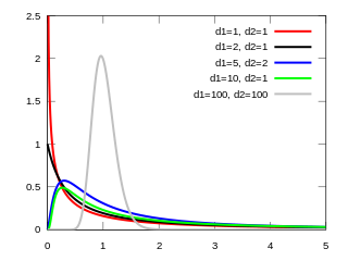
In probability theory and statistics, the F-distribution or F-ratio, also known as Snedecor's F distribution or the Fisher–Snedecor distribution, is a continuous probability distribution that arises frequently as the null distribution of a test statistic, most notably in the analysis of variance (ANOVA) and other F-tests.

In probability theory and statistics, the Laplace distribution is a continuous probability distribution named after Pierre-Simon Laplace. It is also sometimes called the double exponential distribution, because it can be thought of as two exponential distributions spliced together along the abscissa, although the term is also sometimes used to refer to the Gumbel distribution. The difference between two independent identically distributed exponential random variables is governed by a Laplace distribution, as is a Brownian motion evaluated at an exponentially distributed random time. Increments of Laplace motion or a variance gamma process evaluated over the time scale also have a Laplace distribution.

In probability theory and statistics, the Lévy distribution, named after Paul Lévy, is a continuous probability distribution for a non-negative random variable. In spectroscopy, this distribution, with frequency as the dependent variable, is known as a van der Waals profile. It is a special case of the inverse-gamma distribution. It is a stable distribution.
In probability theory and statistics, the generalized extreme value (GEV) distribution is a family of continuous probability distributions developed within extreme value theory to combine the Gumbel, Fréchet and Weibull families also known as type I, II and III extreme value distributions. By the extreme value theorem the GEV distribution is the only possible limit distribution of properly normalized maxima of a sequence of independent and identically distributed random variables. Note that a limit distribution needs to exist, which requires regularity conditions on the tail of the distribution. Despite this, the GEV distribution is often used as an approximation to model the maxima of long (finite) sequences of random variables.
In information theory, the cross-entropy between two probability distributions and , over the same underlying set of events, measures the average number of bits needed to identify an event drawn from the set when the coding scheme used for the set is optimized for an estimated probability distribution , rather than the true distribution .
In statistics, binomial regression is a regression analysis technique in which the response has a binomial distribution: it is the number of successes in a series of independent Bernoulli trials, where each trial has probability of success . In binomial regression, the probability of a success is related to explanatory variables: the corresponding concept in ordinary regression is to relate the mean value of the unobserved response to explanatory variables.
Expected shortfall (ES) is a risk measure—a concept used in the field of financial risk measurement to evaluate the market risk or credit risk of a portfolio. The "expected shortfall at q% level" is the expected return on the portfolio in the worst of cases. ES is an alternative to value at risk that is more sensitive to the shape of the tail of the loss distribution.
A ratio distribution is a probability distribution constructed as the distribution of the ratio of random variables having two other known distributions. Given two random variables X and Y, the distribution of the random variable Z that is formed as the ratio Z = X/Y is a ratio distribution.
In financial mathematics, tail value at risk (TVaR), also known as tail conditional expectation (TCE) or conditional tail expectation (CTE), is a risk measure associated with the more general value at risk. It quantifies the expected value of the loss given that an event outside a given probability level has occurred.

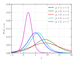
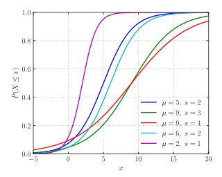
In probability and statistics, the log-logistic distribution is a continuous probability distribution for a non-negative random variable. It is used in survival analysis as a parametric model for events whose rate increases initially and decreases later, as, for example, mortality rate from cancer following diagnosis or treatment. It has also been used in hydrology to model stream flow and precipitation, in economics as a simple model of the distribution of wealth or income, and in networking to model the transmission times of data considering both the network and the software.
The term generalized logistic distribution is used as the name for several different families of probability distributions. For example, Johnson et al. list four forms, which are listed below.

In probability theory and statistics, the Poisson distribution is a discrete probability distribution that expresses the probability of a given number of events occurring in a fixed interval of time if these events occur with a known constant mean rate and independently of the time since the last event. It can also be used for the number of events in other types of intervals than time, and in dimension greater than 1.
In statistics, the variance function is a smooth function that depicts the variance of a random quantity as a function of its mean. The variance function is a measure of heteroscedasticity and plays a large role in many settings of statistical modelling. It is a main ingredient in the generalized linear model framework and a tool used in non-parametric regression, semiparametric regression and functional data analysis. In parametric modeling, variance functions take on a parametric form and explicitly describe the relationship between the variance and the mean of a random quantity. In a non-parametric setting, the variance function is assumed to be a smooth function.