Laplace distribution

Last updated
Laplace
Probability density function
Laplace pdf mod.svg
Cumulative distribution function
Laplace cdf mod.svg
Parameters location (real)
scale (real)
Support
PDF
CDF
Quantile
Mean
Median
Mode
Variance
MAD
Skewness
Excess kurtosis
Entropy
MGF
CF
Expected shortfall [1]

In probability theory and statistics, the Laplace distribution is a continuous probability distribution named after Pierre-Simon Laplace. It is also sometimes called the double exponential distribution, because it can be thought of as two exponential distributions (with an additional location parameter) spliced together along the abscissa, although the term is also sometimes used to refer to the Gumbel distribution. The difference between two independent identically distributed exponential random variables is governed by a Laplace distribution, as is a Brownian motion evaluated at an exponentially distributed random time[ citation needed ]. Increments of Laplace motion or a variance gamma process evaluated over the time scale also have a Laplace distribution.

Contents

Definitions

Probability density function

A random variable has a distribution if its probability density function is

where is a location parameter, and , which is sometimes referred to as the "diversity", is a scale parameter. If and , the positive half-line is exactly an exponential distribution scaled by 1/2.

The probability density function of the Laplace distribution is also reminiscent of the normal distribution; however, whereas the normal distribution is expressed in terms of the squared difference from the mean , the Laplace density is expressed in terms of the absolute difference from the mean. Consequently, the Laplace distribution has fatter tails than the normal distribution. It is a special case of the generalized normal distribution and the hyperbolic distribution. Continuous symmetric distributions that have exponential tails, like the Laplace distribution, but which have probability density functions that are differentiable at the mode include the logistic distribution, hyperbolic secant distribution, and the Champernowne distribution.

Cumulative distribution function

The Laplace distribution is easy to integrate (if one distinguishes two symmetric cases) due to the use of the absolute value function. Its cumulative distribution function is as follows:

The inverse cumulative distribution function is given by

Properties

Moments

Probability of a Laplace being greater than another

Let be independent laplace random variables: and , and we want to compute .

The probability of can be reduced (using the properties below) to , where . This probability is equal to

When , both expressions are replaced by their limit as :

To compute the case for , note that

since when

Relation to the exponential distribution

A Laplace random variable can be represented as the difference of two independent and identically distributed (iid) exponential random variables. [2] One way to show this is by using the characteristic function approach. For any set of independent continuous random variables, for any linear combination of those variables, its characteristic function (which uniquely determines the distribution) can be acquired by multiplying the corresponding characteristic functions.

Consider two i.i.d random variables . The characteristic functions for are

respectively. On multiplying these characteristic functions (equivalent to the characteristic function of the sum of the random variables ), the result is

This is the same as the characteristic function for , which is

Sargan distributions

Sargan distributions are a system of distributions of which the Laplace distribution is a core member. A th order Sargan distribution has density [3] [4]

for parameters . The Laplace distribution results for .

Statistical inference

Given independent and identically distributed samples , the maximum likelihood (MLE) estimator of is the sample median, [5]

The MLE estimator of is the mean absolute deviation from the median,[ citation needed ]

revealing a link between the Laplace distribution and least absolute deviations. A correction for small samples can be applied as follows:

(see: exponential distribution#Parameter estimation).

Occurrence and applications

The Laplacian distribution has been used in speech recognition to model priors on DFT coefficients [6] and in JPEG image compression to model AC coefficients [7] generated by a DCT.

Fitted Laplace distribution to maximum one-day rainfalls Laplace Surinam.png
Fitted Laplace distribution to maximum one-day rainfalls
The Laplace distribution, being a composite or double distribution, is applicable in situations where the lower values originate under different external conditions than the higher ones so that they follow a different pattern. [12]

Random variate generation

Given a random variable drawn from the uniform distribution in the interval , the random variable

has a Laplace distribution with parameters and . This follows from the inverse cumulative distribution function given above.

A variate can also be generated as the difference of two i.i.d. random variables. Equivalently, can also be generated as the logarithm of the ratio of two i.i.d. uniform random variables.

History

This distribution is often referred to as "Laplace's first law of errors". He published it in 1774, modeling the frequency of an error as an exponential function of its magnitude once its sign was disregarded. Laplace would later replace this model with his "second law of errors", based on the normal distribution, after the discovery of the central limit theorem. [13] [14]

Keynes published a paper in 1911 based on his earlier thesis wherein he showed that the Laplace distribution minimised the absolute deviation from the median. [15]

See also

Related Research Articles

<span class="mw-page-title-main">Normal distribution</span> Probability distribution

In probability theory and statistics, a normal distribution or Gaussian distribution is a type of continuous probability distribution for a real-valued random variable. The general form of its probability density function is

<span class="mw-page-title-main">Exponential distribution</span> Probability distribution

In probability theory and statistics, the exponential distribution or negative exponential distribution is the probability distribution of the distance between events in a Poisson point process, i.e., a process in which events occur continuously and independently at a constant average rate; the distance parameter could be any meaningful mono-dimensional measure of the process, such as time between production errors, or length along a roll of fabric in the weaving manufacturing process. It is a particular case of the gamma distribution. It is the continuous analogue of the geometric distribution, and it has the key property of being memoryless. In addition to being used for the analysis of Poisson point processes it is found in various other contexts.

<span class="mw-page-title-main">Chi-squared distribution</span> Probability distribution and special case of gamma distribution

In probability theory and statistics, the chi-squared distribution with degrees of freedom is the distribution of a sum of the squares of independent standard normal random variables. The chi-squared distribution is a special case of the gamma distribution and is one of the most widely used probability distributions in inferential statistics, notably in hypothesis testing and in construction of confidence intervals. This distribution is sometimes called the central chi-squared distribution, a special case of the more general noncentral chi-squared distribution.

<span class="mw-page-title-main">Weibull distribution</span> Continuous probability distribution

In probability theory and statistics, the Weibull distribution is a continuous probability distribution. It models a broad range of random variables, largely in the nature of a time to failure or time between events. Examples are maximum one-day rainfalls and the time a user spends on a web page.

In probability theory, a compound Poisson distribution is the probability distribution of the sum of a number of independent identically-distributed random variables, where the number of terms to be added is itself a Poisson-distributed variable. The result can be either a continuous or a discrete distribution.

In probability theory and statistics, the generalized extreme value (GEV) distribution is a family of continuous probability distributions developed within extreme value theory to combine the Gumbel, Fréchet and Weibull families also known as type I, II and III extreme value distributions. By the extreme value theorem the GEV distribution is the only possible limit distribution of properly normalized maxima of a sequence of independent and identically distributed random variables. Note that a limit distribution needs to exist, which requires regularity conditions on the tail of the distribution. Despite this, the GEV distribution is often used as an approximation to model the maxima of long (finite) sequences of random variables.

In statistics and information theory, a maximum entropy probability distribution has entropy that is at least as great as that of all other members of a specified class of probability distributions. According to the principle of maximum entropy, if nothing is known about a distribution except that it belongs to a certain class, then the distribution with the largest entropy should be chosen as the least-informative default. The motivation is twofold: first, maximizing entropy minimizes the amount of prior information built into the distribution; second, many physical systems tend to move towards maximal entropy configurations over time.

<span class="mw-page-title-main">Noncentral chi-squared distribution</span> Noncentral generalization of the chi-squared distribution

In probability theory and statistics, the noncentral chi-squared distribution is a noncentral generalization of the chi-squared distribution. It often arises in the power analysis of statistical tests in which the null distribution is a chi-squared distribution; important examples of such tests are the likelihood-ratio tests.

<span class="mw-page-title-main">Inverse Gaussian distribution</span> Family of continuous probability distributions

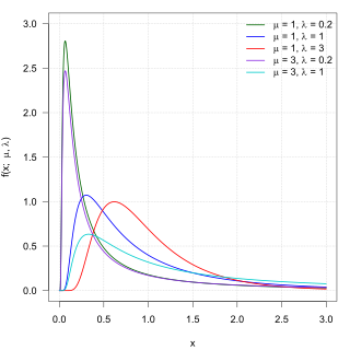
In probability theory, the inverse Gaussian distribution is a two-parameter family of continuous probability distributions with support on (0,∞).

A ratio distribution is a probability distribution constructed as the distribution of the ratio of random variables having two other known distributions. Given two random variables X and Y, the distribution of the random variable Z that is formed as the ratio Z = X/Y is a ratio distribution.

In probability theory and statistics, the normal-gamma distribution is a bivariate four-parameter family of continuous probability distributions. It is the conjugate prior of a normal distribution with unknown mean and precision.

In probability and statistics, the Tweedie distributions are a family of probability distributions which include the purely continuous normal, gamma and inverse Gaussian distributions, the purely discrete scaled Poisson distribution, and the class of compound Poisson–gamma distributions which have positive mass at zero, but are otherwise continuous. Tweedie distributions are a special case of exponential dispersion models and are often used as distributions for generalized linear models.

In probability and statistics, the class of exponential dispersion models (EDM), also called exponential dispersion family (EDF), is a set of probability distributions that represents a generalisation of the natural exponential family. Exponential dispersion models play an important role in statistical theory, in particular in generalized linear models because they have a special structure which enables deductions to be made about appropriate statistical inference.

<span class="mw-page-title-main">Normal-inverse-gamma distribution</span>

In probability theory and statistics, the normal-inverse-gamma distribution is a four-parameter family of multivariate continuous probability distributions. It is the conjugate prior of a normal distribution with unknown mean and variance.

Financial models with long-tailed distributions and volatility clustering have been introduced to overcome problems with the realism of classical financial models. These classical models of financial time series typically assume homoskedasticity and normality cannot explain stylized phenomena such as skewness, heavy tails, and volatility clustering of the empirical asset returns in finance. In 1963, Benoit Mandelbrot first used the stable distribution to model the empirical distributions which have the skewness and heavy-tail property. Since -stable distributions have infinite -th moments for all , the tempered stable processes have been proposed for overcoming this limitation of the stable distribution.

<span class="mw-page-title-main">Poisson distribution</span> Discrete probability distribution

In probability theory and statistics, the Poisson distribution is a discrete probability distribution that expresses the probability of a given number of events occurring in a fixed interval of time if these events occur with a known constant mean rate and independently of the time since the last event. It can also be used for the number of events in other types of intervals than time, and in dimension greater than 1.

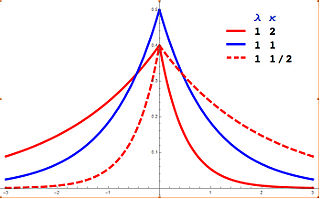
A geometric stable distribution or geo-stable distribution is a type of leptokurtic probability distribution. Geometric stable distributions were introduced in Klebanov, L. B., Maniya, G. M., and Melamed, I. A. (1985). A problem of Zolotarev and analogs of infinitely divisible and stable distributions in a scheme for summing a random number of random variables. These distributions are analogues for stable distributions for the case when the number of summands is random, independent of the distribution of summand, and having geometric distribution. The geometric stable distribution may be symmetric or asymmetric. A symmetric geometric stable distribution is also referred to as a Linnik distribution. The Laplace distribution and asymmetric Laplace distribution are special cases of the geometric stable distribution. The Mittag-Leffler distribution is also a special case of a geometric stable distribution.

<i>q</i>-exponential distribution

The q-exponential distribution is a probability distribution arising from the maximization of the Tsallis entropy under appropriate constraints, including constraining the domain to be positive. It is one example of a Tsallis distribution. The q-exponential is a generalization of the exponential distribution in the same way that Tsallis entropy is a generalization of standard Boltzmann–Gibbs entropy or Shannon entropy. The exponential distribution is recovered as

In probability theory and statistics, the noncentral beta distribution is a continuous probability distribution that is a noncentral generalization of the (central) beta distribution.

<span class="mw-page-title-main">Asymmetric Laplace distribution</span> Continuous probability distribution

In probability theory and statistics, the asymmetric Laplace distribution (ALD) is a continuous probability distribution which is a generalization of the Laplace distribution. Just as the Laplace distribution consists of two exponential distributions of equal scale back-to-back about x = m, the asymmetric Laplace consists of two exponential distributions of unequal scale back to back about x = m, adjusted to assure continuity and normalization. The difference of two variates exponentially distributed with different means and rate parameters will be distributed according to the ALD. When the two rate parameters are equal, the difference will be distributed according to the Laplace distribution.

References

  1. Norton, Matthew; Khokhlov, Valentyn; Uryasev, Stan (2019). "Calculating CVaR and bPOE for common probability distributions with application to portfolio optimization and density estimation" (PDF). Annals of Operations Research. 299 (1–2). Springer: 1281–1315. doi:10.1007/s10479-019-03373-1 . Retrieved 2023-02-27.
  2. 1 2 Kotz, Samuel; Kozubowski, Tomasz J.; Podgórski, Krzysztof (2001). The Laplace distribution and generalizations: a revisit with applications to Communications, Economics, Engineering and Finance. Birkhauser. pp. 23 (Proposition 2.2.2, Equation 2.2.8). ISBN   9780817641665.
  3. Everitt, B.S. (2002) The Cambridge Dictionary of Statistics, CUP. ISBN   0-521-81099-X
  4. Johnson, N.L., Kotz S., Balakrishnan, N. (1994) Continuous Univariate Distributions, Wiley. ISBN   0-471-58495-9. p. 60
  5. Robert M. Norton (May 1984). "The Double Exponential Distribution: Using Calculus to Find a Maximum Likelihood Estimator". The American Statistician . 38 (2). American Statistical Association: 135–136. doi:10.2307/2683252. JSTOR   2683252.
  6. Eltoft, T.; Taesu Kim; Te-Won Lee (2006). "On the multivariate Laplace distribution" (PDF). IEEE Signal Processing Letters. 13 (5): 300–303. doi:10.1109/LSP.2006.870353. S2CID   1011487. Archived from the original (PDF) on 2013-06-06. Retrieved 2012-07-04.
  7. Minguillon, J.; Pujol, J. (2001). "JPEG standard uniform quantization error modeling with applications to sequential and progressive operation modes" (PDF). Journal of Electronic Imaging. 10 (2): 475–485. doi:10.1117/1.1344592. hdl: 10609/6263 .
  8. CumFreq for probability distribution fitting
  9. Pardo, Scott (2020). Statistical Analysis of Empirical Data Methods for Applied Sciences. Springer. p. 58. ISBN   978-3-030-43327-7.
  10. Kou, S.G. (August 8, 2002). "A Jump-Diffusion Model for Option Pricing". Management Science. 48 (8): 1086–1101. doi:10.1287/mnsc.48.8.1086.166. JSTOR   822677 . Retrieved 2022-03-01.
  11. Chen, Jian (2018). General Equilibrium Option Pricing Method: Theoretical and Empirical Study. Springer. p. 70. ISBN   9789811074288.
  12. A collection of composite distributions
  13. Laplace, P-S. (1774). Mémoire sur la probabilité des causes par les évènements. Mémoires de l’Academie Royale des Sciences Presentés par Divers Savan, 6, 621–656
  14. Wilson, Edwin Bidwell (1923). "First and Second Laws of Error". Journal of the American Statistical Association. 18 (143). Informa UK Limited: 841–851. doi:10.1080/01621459.1923.10502116. ISSN   0162-1459.PD-icon.svg This article incorporates text from this source, which is in the public domain .
  15. Keynes, J. M. (1911). "The Principal Averages and the Laws of Error which Lead to Them". Journal of the Royal Statistical Society. 74 (3). JSTOR: 322–331. doi:10.2307/2340444. ISSN   0952-8385. JSTOR   2340444.