Skewness

Last updated

Example distribution with positive skewness. These data are from experiments on wheat grass growth. SkewedDistribution.png
Example distribution with positive skewness. These data are from experiments on wheat grass growth.

In probability theory and statistics, skewness is a measure of the asymmetry of the probability distribution of a real-valued random variable about its mean. The skewness value can be positive, zero, negative, or undefined.

Contents

For a unimodal distribution (a distribution with a single peak), negative skew commonly indicates that the tail is on the left side of the distribution, and positive skew indicates that the tail is on the right. In cases where one tail is long but the other tail is fat, skewness does not obey a simple rule. For example, a zero value in skewness means that the tails on both sides of the mean balance out overall; this is the case for a symmetric distribution but can also be true for an asymmetric distribution where one tail is long and thin, and the other is short but fat. Thus, the judgement on the symmetry of a given distribution by using only its skewness is risky; the distribution shape must be taken into account.

Introduction

Consider the two distributions in the figure just below. Within each graph, the values on the right side of the distribution taper differently from the values on the left side. These tapering sides are called tails, and they provide a visual means to determine which of the two kinds of skewness a distribution has:

  1. negative skew: The left tail is longer; the mass of the distribution is concentrated on the right of the figure. The distribution is said to be left-skewed, left-tailed, or skewed to the left, despite the fact that the curve itself appears to be skewed or leaning to the right; left instead refers to the left tail being drawn out and, often, the mean being skewed to the left of a typical center of the data. A left-skewed distribution usually appears as a right-leaning curve. [1]
  2. positive skew: The right tail is longer; the mass of the distribution is concentrated on the left of the figure. The distribution is said to be right-skewed, right-tailed, or skewed to the right, despite the fact that the curve itself appears to be skewed or leaning to the left; right instead refers to the right tail being drawn out and, often, the mean being skewed to the right of a typical center of the data. A right-skewed distribution usually appears as a left-leaning curve. [1]

Negative and positive skew diagrams (English).svg

Skewness in a data series may sometimes be observed not only graphically but by simple inspection of the values. For instance, consider the numeric sequence (49, 50, 51), whose values are evenly distributed around a central value of 50. We can transform this sequence into a negatively skewed distribution by adding a value far below the mean, which is probably a negative outlier, e.g. (40, 49, 50, 51). Therefore, the mean of the sequence becomes 47.5, and the median is 49.5. Based on the formula of nonparametric skew, defined as the skew is negative. Similarly, we can make the sequence positively skewed by adding a value far above the mean, which is probably a positive outlier, e.g. (49, 50, 51, 60), where the mean is 52.5, and the median is 50.5.

As mentioned earlier, a unimodal distribution with zero value of skewness does not imply that this distribution is symmetric necessarily. However, a symmetric unimodal or multimodal distribution always has zero skewness.

Example of an asymmetric distribution with zero skewness. This figure serves as a counterexample that zero skewness does not imply symmetric distribution necessarily. (Skewness was calculated by Pearson's moment coefficient of skewness.) Asymmetric Distribution with Zero Skewness.jpg
Example of an asymmetric distribution with zero skewness. This figure serves as a counterexample that zero skewness does not imply symmetric distribution necessarily. (Skewness was calculated by Pearson's moment coefficient of skewness.)

Relationship of mean and median

The skewness is not directly related to the relationship between the mean and median: a distribution with negative skew can have its mean greater than or less than the median, and likewise for positive skew. [2]

A general relationship of mean and median under differently skewed unimodal distribution. Relationship between mean and median under different skewness.png
A general relationship of mean and median under differently skewed unimodal distribution.

In the older notion of nonparametric skew, defined as where is the mean, is the median, and is the standard deviation, the skewness is defined in terms of this relationship: positive/right nonparametric skew means the mean is greater than (to the right of) the median, while negative/left nonparametric skew means the mean is less than (to the left of) the median. However, the modern definition of skewness and the traditional nonparametric definition do not always have the same sign: while they agree for some families of distributions, they differ in some of the cases, and conflating them is misleading.

If the distribution is symmetric, then the mean is equal to the median, and the distribution has zero skewness. [3] If the distribution is both symmetric and unimodal, then the mean = median = mode. This is the case of a coin toss or the series 1,2,3,4,... Note, however, that the converse is not true in general, i.e. zero skewness (defined below) does not imply that the mean is equal to the median.

A 2005 journal article points out: [2]

Many textbooks teach a rule of thumb stating that the mean is right of the median under right skew, and left of the median under left skew. This rule fails with surprising frequency. It can fail in multimodal distributions, or in distributions where one tail is long but the other is heavy. Most commonly, though, the rule fails in discrete distributions where the areas to the left and right of the median are not equal. Such distributions not only contradict the textbook relationship between mean, median, and skew, they also contradict the textbook interpretation of the median.

Distribution of adult residents across US households Positive skewness with mean less than median.png
Distribution of adult residents across US households

For example, in the distribution of adult residents across US households, the skew is to the right. However, since the majority of cases is less than or equal to the mode, which is also the median, the mean sits in the heavier left tail. As a result, the rule of thumb that the mean is right of the median under right skew failed. [2]

Definition

Fisher's moment coefficient of skewness

The skewness of a random variable X is the third standardized moment , defined as: [4] [5]

where μ is the mean, σ is the standard deviation, E is the expectation operator, μ3 is the third central moment, and κt are the t-th cumulants. It is sometimes referred to as Pearson's moment coefficient of skewness, [5] or simply the moment coefficient of skewness, [4] but should not be confused with Pearson's other skewness statistics (see below). The last equality expresses skewness in terms of the ratio of the third cumulant κ3 to the 1.5th power of the second cumulant κ2. This is analogous to the definition of kurtosis as the fourth cumulant normalized by the square of the second cumulant. The skewness is also sometimes denoted Skew[X].

If σ is finite and μ is finite too, then skewness can be expressed in terms of the non-central moment E[X3] by expanding the previous formula:

Examples

Skewness can be infinite, as when

where the third cumulants are infinite, or as when

where the third cumulant is undefined.

Examples of distributions with finite skewness include the following.

Sample skewness

For a sample of n values, two natural estimators of the population skewness are [6]

and

where is the sample mean, s is the sample standard deviation, m2 is the (biased) sample second central moment, and m3 is the (biased) sample third central moment. [6] is a method of moments estimator.

Another common definition of the sample skewness is [6] [7]

where is the unique symmetric unbiased estimator of the third cumulant and is the symmetric unbiased estimator of the second cumulant (i.e. the sample variance). This adjusted Fisher–Pearson standardized moment coefficient is the version found in Excel and several statistical packages including Minitab, SAS and SPSS. [7]

Under the assumption that the underlying random variable is normally distributed, it can be shown that all three ratios , and are unbiased and consistent estimators of the population skewness , with , i.e., their distributions converge to a normal distribution with mean 0 and variance 6 (Fisher, 1930). [6] The variance of the sample skewness is thus approximately for sufficiently large samples. More precisely, in a random sample of size n from a normal distribution, [8] [9]

In normal samples, has the smaller variance of the three estimators, with [6]

For non-normal distributions, , and are generally biased estimators of the population skewness ; their expected values can even have the opposite sign from the true skewness. For instance, a mixed distribution consisting of very thin Gaussians centred at −99, 0.5, and 2 with weights 0.01, 0.66, and 0.33 has a skewness of about −9.77, but in a sample of 3 has an expected value of about 0.32, since usually all three samples are in the positive-valued part of the distribution, which is skewed the other way.

Applications

Skewness is a descriptive statistic that can be used in conjunction with the histogram and the normal quantile plot to characterize the data or distribution.

Skewness indicates the direction and relative magnitude of a distribution's deviation from the normal distribution.

With pronounced skewness, standard statistical inference procedures such as a confidence interval for a mean will be not only incorrect, in the sense that the true coverage level will differ from the nominal (e.g., 95%) level, but they will also result in unequal error probabilities on each side.

Skewness can be used to obtain approximate probabilities and quantiles of distributions (such as value at risk in finance) via the Cornish–Fisher expansion.

Many models assume normal distribution; i.e., data are symmetric about the mean. The normal distribution has a skewness of zero. But in reality, data points may not be perfectly symmetric. So, an understanding of the skewness of the dataset indicates whether deviations from the mean are going to be positive or negative.

D'Agostino's K-squared test is a goodness-of-fit normality test based on sample skewness and sample kurtosis.

Other measures of skewness

Comparison of mean, median and mode of two log-normal distributions with the same medians and different skewnesses. Comparison mean median mode.svg
Comparison of mean, median and mode of two log-normal distributions with the same medians and different skewnesses.

Other measures of skewness have been used, including simpler calculations suggested by Karl Pearson [10] (not to be confused with Pearson's moment coefficient of skewness, see above). These other measures are:

Pearson's first skewness coefficient (mode skewness)

The Pearson mode skewness, [11] or first skewness coefficient, is defined as

meanmode / standard deviation .

Pearson's second skewness coefficient (median skewness)

The Pearson median skewness, or second skewness coefficient, [12] [13] is defined as

3 (meanmedian)/ standard deviation .

Which is a simple multiple of the nonparametric skew.

Quantile-based measures

Bowley's measure of skewness (from 1901), [14] [15] also called Yule's coefficient (from 1912) [16] [17] is defined as:

where Q is the quantile function (i.e., the inverse of the cumulative distribution function). The numerator is difference between the average of the upper and lower quartiles (a measure of location) and the median (another measure of location), while the denominator is the semi-interquartile range , which for symmetric distributions is the MAD measure of dispersion.

Other names for this measure are Galton's measure of skewness, [18] the Yule–Kendall index [19] and the quartile skewness, [20]

Similarly, Kelly's measure of skewness is defined as [21]

A more general formulation of a skewness function was described by Groeneveld, R. A. and Meeden, G. (1984): [22] [23] [24]

The function γ(u) satisfies −1  γ(u)  1 and is well defined without requiring the existence of any moments of the distribution. [22] Bowley's measure of skewness is γ(u) evaluated at u = 3/4 while Kelly's measure of skewness is γ(u) evaluated at u = 9/10. This definition leads to a corresponding overall measure of skewness [23] defined as the supremum of this over the range 1/2  u < 1. Another measure can be obtained by integrating the numerator and denominator of this expression. [22]

Quantile-based skewness measures are at first glance easy to interpret, but they often show significantly larger sample variations than moment-based methods. This means that often samples from a symmetric distribution (like the uniform distribution) have a large quantile-based skewness, just by chance.

Groeneveld and Meeden's coefficient

Groeneveld and Meeden have suggested, as an alternative measure of skewness, [22]

where μ is the mean, ν is the median, |...| is the absolute value, and E() is the expectation operator. This is closely related in form to Pearson's second skewness coefficient.

L-moments

Use of L-moments in place of moments provides a measure of skewness known as the L-skewness. [25]

Distance skewness

A value of skewness equal to zero does not imply that the probability distribution is symmetric. Thus there is a need for another measure of asymmetry that has this property: such a measure was introduced in 2000. [26] It is called distance skewness and denoted by dSkew. If X is a random variable taking values in the d-dimensional Euclidean space, X has finite expectation, X' is an independent identically distributed copy of X, and denotes the norm in the Euclidean space, then a simple measure of asymmetry with respect to location parameter θ is

and dSkew(X) := 0 for X = θ (with probability 1). Distance skewness is always between 0 and 1, equals 0 if and only if X is diagonally symmetric with respect to θ (X and 2θ−X have the same probability distribution) and equals 1 if and only if X is a constant c () with probability one. [27] Thus there is a simple consistent statistical test of diagonal symmetry based on the sample distance skewness:

Medcouple

The medcouple is a scale-invariant robust measure of skewness, with a breakdown point of 25%. [28] It is the median of the values of the kernel function

taken over all couples such that , where is the median of the sample . It can be seen as the median of all possible quantile skewness measures.

See also

Related Research Articles

In probability theory and statistics, kurtosis is a measure of the "tailedness" of the probability distribution of a real-valued random variable. Like skewness, kurtosis describes a particular aspect of a probability distribution. There are different ways to quantify kurtosis for a theoretical distribution, and there are corresponding ways of estimating it using a sample from a population. Different measures of kurtosis may have different interpretations.

In probability theory and statistics, a central moment is a moment of a probability distribution of a random variable about the random variable's mean; that is, it is the expected value of a specified integer power of the deviation of the random variable from the mean. The various moments form one set of values by which the properties of a probability distribution can be usefully characterized. Central moments are used in preference to ordinary moments, computed in terms of deviations from the mean instead of from zero, because the higher-order central moments relate only to the spread and shape of the distribution, rather than also to its location.

<span class="mw-page-title-main">Normal distribution</span> Probability distribution

In probability theory and statistics, a normal distribution or Gaussian distribution is a type of continuous probability distribution for a real-valued random variable. The general form of its probability density function is

<span class="mw-page-title-main">Standard deviation</span> In statistics, a measure of variation

In statistics, the standard deviation is a measure of the amount of variation of a random variable expected about its mean. A low standard deviation indicates that the values tend to be close to the mean of the set, while a high standard deviation indicates that the values are spread out over a wider range. The standard deviation is commonly used in the determination of what constitutes an outlier and what does not.

<span class="mw-page-title-main">Variance</span> Statistical measure of how far values spread from their average

In probability theory and statistics, variance is the expected value of the squared deviation from the mean of a random variable. The standard deviation (SD) is obtained as the square root of the variance. Variance is a measure of dispersion, meaning it is a measure of how far a set of numbers is spread out from their average value. It is the second central moment of a distribution, and the covariance of the random variable with itself, and it is often represented by , , , , or .

<span class="mw-page-title-main">Multivariate normal distribution</span> Generalization of the one-dimensional normal distribution to higher dimensions

In probability theory and statistics, the multivariate normal distribution, multivariate Gaussian distribution, or joint normal distribution is a generalization of the one-dimensional (univariate) normal distribution to higher dimensions. One definition is that a random vector is said to be k-variate normally distributed if every linear combination of its k components has a univariate normal distribution. Its importance derives mainly from the multivariate central limit theorem. The multivariate normal distribution is often used to describe, at least approximately, any set of (possibly) correlated real-valued random variables, each of which clusters around a mean value.

<span class="mw-page-title-main">Log-normal distribution</span> Probability distribution

In probability theory, a log-normal (or lognormal) distribution is a continuous probability distribution of a random variable whose logarithm is normally distributed. Thus, if the random variable X is log-normally distributed, then Y = ln(X) has a normal distribution. Equivalently, if Y has a normal distribution, then the exponential function of Y, X = exp(Y), has a log-normal distribution. A random variable which is log-normally distributed takes only positive real values. It is a convenient and useful model for measurements in exact and engineering sciences, as well as medicine, economics and other topics (e.g., energies, concentrations, lengths, prices of financial instruments, and other metrics).

In probability theory, Chebyshev's inequality provides an upper bound on the probability of deviation of a random variable from its mean. More specifically, the probability that a random variable deviates from its mean by more than is at most , where is any positive constant and is the standard deviation.

<span class="mw-page-title-main">Bernoulli distribution</span> Probability distribution modeling a coin toss which need not be fair

In probability theory and statistics, the Bernoulli distribution, named after Swiss mathematician Jacob Bernoulli, is the discrete probability distribution of a random variable which takes the value 1 with probability and the value 0 with probability . Less formally, it can be thought of as a model for the set of possible outcomes of any single experiment that asks a yes–no question. Such questions lead to outcomes that are Boolean-valued: a single bit whose value is success/yes/true/one with probability p and failure/no/false/zero with probability q. It can be used to represent a coin toss where 1 and 0 would represent "heads" and "tails", respectively, and p would be the probability of the coin landing on heads. In particular, unfair coins would have

In statistics, the mean squared error (MSE) or mean squared deviation (MSD) of an estimator measures the average of the squares of the errors—that is, the average squared difference between the estimated values and the actual value. MSE is a risk function, corresponding to the expected value of the squared error loss. The fact that MSE is almost always strictly positive is because of randomness or because the estimator does not account for information that could produce a more accurate estimate. In machine learning, specifically empirical risk minimization, MSE may refer to the empirical risk, as an estimate of the true MSE.

<span class="mw-page-title-main">Beta distribution</span> Probability distribution

In probability theory and statistics, the beta distribution is a family of continuous probability distributions defined on the interval [0, 1] or in terms of two positive parameters, denoted by alpha (α) and beta (β), that appear as exponents of the variable and its complement to 1, respectively, and control the shape of the distribution.

In mathematics, the moments of a function are certain quantitative measures related to the shape of the function's graph. If the function represents mass density, then the zeroth moment is the total mass, the first moment is the center of mass, and the second moment is the moment of inertia. If the function is a probability distribution, then the first moment is the expected value, the second central moment is the variance, the third standardized moment is the skewness, and the fourth standardized moment is the kurtosis. The mathematical concept is closely related to the concept of moment in physics.

In probability theory and statistics, the generalized extreme value (GEV) distribution is a family of continuous probability distributions developed within extreme value theory to combine the Gumbel, Fréchet and Weibull families also known as type I, II and III extreme value distributions. By the extreme value theorem the GEV distribution is the only possible limit distribution of properly normalized maxima of a sequence of independent and identically distributed random variables. Note that a limit distribution needs to exist, which requires regularity conditions on the tail of the distribution. Despite this, the GEV distribution is often used as an approximation to model the maxima of long (finite) sequences of random variables.

<span class="mw-page-title-main">Pearson distribution</span> Family of continuous probability distributions

The Pearson distribution is a family of continuous probability distributions. It was first published by Karl Pearson in 1895 and subsequently extended by him in 1901 and 1916 in a series of articles on biostatistics.

In statistics, the bias of an estimator is the difference between this estimator's expected value and the true value of the parameter being estimated. An estimator or decision rule with zero bias is called unbiased. In statistics, "bias" is an objective property of an estimator. Bias is a distinct concept from consistency: consistent estimators converge in probability to the true value of the parameter, but may be biased or unbiased; see bias versus consistency for more.

In statistics, D'Agostino's K2 test, named for Ralph D'Agostino, is a goodness-of-fit measure of departure from normality, that is the test aims to gauge the compatibility of given data with the null hypothesis that the data is a realization of independent, identically distributed Gaussian random variables. The test is based on transformations of the sample kurtosis and skewness, and has power only against the alternatives that the distribution is skewed and/or kurtic.

In statistics, the Jarque–Bera test is a goodness-of-fit test of whether sample data have the skewness and kurtosis matching a normal distribution. The test is named after Carlos Jarque and Anil K. Bera. The test statistic is always nonnegative. If it is far from zero, it signals the data do not have a normal distribution.

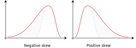
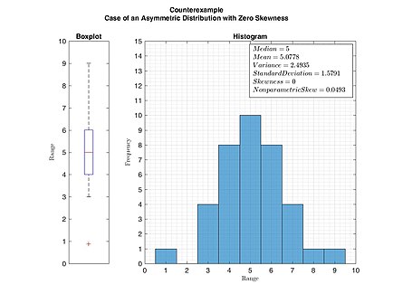
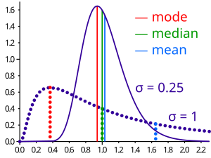
In statistics and probability theory, the nonparametric skew is a statistic occasionally used with random variables that take real values. It is a measure of the skewness of a random variable's distribution—that is, the distribution's tendency to "lean" to one side or the other of the mean. Its calculation does not require any knowledge of the form of the underlying distribution—hence the name nonparametric. It has some desirable properties: it is zero for any symmetric distribution; it is unaffected by a scale shift; and it reveals either left- or right-skewness equally well. In some statistical samples it has been shown to be less powerful than the usual measures of skewness in detecting departures of the population from normality.

<span class="mw-page-title-main">Hermite distribution</span> Statistical probability Distribution for discrete event counts

In probability theory and statistics, the Hermite distribution, named after Charles Hermite, is a discrete probability distribution used to model count data with more than one parameter. This distribution is flexible in terms of its ability to allow a moderate over-dispersion in the data.

In probability and statistics, the skewed generalized "t" distribution is a family of continuous probability distributions. The distribution was first introduced by Panayiotis Theodossiou in 1998. The distribution has since been used in different applications. There are different parameterizations for the skewed generalized t distribution.

References

Citations

  1. 1 2 Illowsky, Barbara; Dean, Susan (27 March 2020). "2.6 Skewness and the Mean, Median, and Mode – Statistics". OpenStax . Retrieved 21 December 2022.
  2. 1 2 3 von Hippel, Paul T. (2005). "Mean, Median, and Skew: Correcting a Textbook Rule". Journal of Statistics Education. 13 (2). Archived from the original on 20 February 2016.
  3. "1.3.5.11. Measures of Skewness and Kurtosis". NIST. Retrieved 18 March 2012.
  4. 1 2 "Measures of Shape: Skewness and Kurtosis", 2008–2016 by Stan Brown, Oak Road Systems
  5. 1 2 Pearson's moment coefficient of skewness, FXSolver.com
  6. 1 2 3 4 5 Joanes, D. N.; Gill, C. A. (1998). "Comparing measures of sample skewness and kurtosis". Journal of the Royal Statistical Society, Series D . 47 (1): 183–189. doi:10.1111/1467-9884.00122.
  7. 1 2 Doane, David P., and Lori E. Seward. "Measuring skewness: a forgotten statistic." Journal of Statistics Education 19.2 (2011): 1-18. (Page 7)
  8. Duncan Cramer (1997) Fundamental Statistics for Social Research. Routledge. ISBN   9780415172042 (p 85)
  9. Kendall, M.G.; Stuart, A. (1969) The Advanced Theory of Statistics, Volume 1: Distribution Theory, 3rd Edition, Griffin. ISBN   0-85264-141-9 (Ex 12.9)
  10. "Archived copy" (PDF). Archived from the original (PDF) on 5 July 2010. Retrieved 9 April 2010.{{cite web}}: CS1 maint: archived copy as title (link)
  11. Weisstein, Eric W. "Pearson Mode Skewness". MathWorld .
  12. Weisstein, Eric W. "Pearson's skewness coefficients". MathWorld .
  13. Doane, David P.; Seward, Lori E. (2011). "Measuring Skewness: A Forgotten Statistic?" (PDF). Journal of Statistics Education. 19 (2): 1–18. doi: 10.1080/10691898.2011.11889611 .
  14. Bowley, A. L. (1901). Elements of Statistics, P.S. King & Son, Laondon. Or in a later edition: BOWLEY, AL. "Elements of Statistics, 4th Edn (New York, Charles Scribner)."(1920).
  15. Kenney JF and Keeping ES (1962) Mathematics of Statistics, Pt. 1, 3rd ed., Van Nostrand, (page 102).
  16. Yule, George Udny. An introduction to the theory of statistics. C. Griffin, limited, 1912.
  17. Groeneveld, Richard A (1991). "An influence function approach to describing the skewness of a distribution". The American Statistician. 45 (2): 97–102. doi:10.2307/2684367. JSTOR   2684367.
  18. Johnson, NL, Kotz, S & Balakrishnan, N (1994) p. 3 and p. 40
  19. Wilks DS (1995) Statistical Methods in the Atmospheric Sciences, p 27. Academic Press. ISBN   0-12-751965-3
  20. Weisstein, Eric W. "Skewness". mathworld.wolfram.com. Retrieved 21 November 2019.
  21. A.W.L. Pubudu Thilan. "Applied Statistics I: Chapter 5: Measures of skewness" (PDF). University of Ruhuna. p. 21.
  22. 1 2 3 4 Groeneveld, R.A.; Meeden, G. (1984). "Measuring Skewness and Kurtosis". The Statistician. 33 (4): 391–399. doi:10.2307/2987742. JSTOR   2987742.
  23. 1 2 MacGillivray (1992)
  24. Hinkley DV (1975) "On power transformations to symmetry", Biometrika, 62, 101–111
  25. Hosking, J.R.M. (1992). "Moments or L moments? An example comparing two measures of distributional shape". The American Statistician. 46 (3): 186–189. doi:10.2307/2685210. JSTOR   2685210.
  26. Szekely, G.J. (2000). "Pre-limit and post-limit theorems for statistics", In: Statistics for the 21st Century (eds. C. R. Rao and G. J. Szekely), Dekker, New York, pp. 411–422.
  27. Szekely, G. J. and Mori, T. F. (2001) "A characteristic measure of asymmetry and its application for testing diagonal symmetry", Communications in Statistics – Theory and Methods 30/8&9, 1633–1639.
  28. G. Brys; M. Hubert; A. Struyf (November 2004). "A Robust Measure of Skewness". Journal of Computational and Graphical Statistics. 13 (4): 996–1017. doi:10.1198/106186004X12632. S2CID   120919149.

Sources

  • Johnson, NL; Kotz, S; Balakrishnan, N (1994). Continuous Univariate Distributions. Vol. 1 (2 ed.). Wiley. ISBN   0-471-58495-9.
  • MacGillivray, HL (1992). "Shape properties of the g- and h- and Johnson families". Communications in Statistics – Theory and Methods. 21 (5): 1244–1250. doi:10.1080/03610929208830842.
  • Premaratne, G., Bera, A. K. (2001). Adjusting the Tests for Skewness and Kurtosis for Distributional Misspecifications. Working Paper Number 01-0116, University of Illinois. Forthcoming in Comm in Statistics, Simulation and Computation. 2016 1–15
  • Premaratne, G., Bera, A. K. (2000). Modeling Asymmetry and Excess Kurtosis in Stock Return Data. Office of Research Working Paper Number 00-0123, University of Illinois.
  • Skewness Measures for the Weibull Distribution