A wavelet is a wave-like oscillation with an amplitude that begins at zero, increases or decreases, and then returns to zero one or more times. Wavelets are termed a "brief oscillation". A taxonomy of wavelets has been established, based on the number and direction of its pulses. Wavelets are imbued with specific properties that make them useful for signal processing.
For example, a wavelet could be created to have a frequency of Middle C and a short duration of roughly one tenth of a second. If this wavelet were to be convolved with a signal created from the recording of a melody, then the resulting signal would be useful for determining when the MiddleC note appeared in the song. Mathematically, a wavelet correlates with a signal if a portion of the signal is similar. Correlation is at the core of many practical wavelet applications.
As a mathematical tool, wavelets can be used to extract information from many kinds of data, including audio signals and images. Sets of wavelets are needed to analyze data fully. "Complementary" wavelets decompose a signal without gaps or overlaps so that the decomposition process is mathematically reversible. Thus, sets of complementary wavelets are useful in wavelet-based compression/decompression algorithms, where it is desirable to recover the original information with minimal loss.
In classical physics, the diffraction phenomenon is described by the Huygens–Fresnel principle that treats each point in a propagating wavefront as a collection of individual spherical wavelets.[1] The characteristic bending pattern is most pronounced when a wave from a coherent source (such as a laser) encounters a slit/aperture that is comparable in size to its wavelength. This is due to the addition, or interference, of different points on the wavefront (or, equivalently, each wavelet) that travel by paths of different lengths to the registering surface. Multiple, closely spaced openings (e.g., a diffraction grating), can result in a complex pattern of varying intensity.
Etymology
The word wavelet has been used for decades in digital signal processing and exploration geophysics.[2] The equivalent French word ondelette meaning "small wave" was used by Morlet and Grossmann in the early 1980s.
Wavelet theory is applicable to several subjects. All wavelet transforms may be considered forms of time-frequency representation for continuous-time (analog) signals and so are related to harmonic analysis. Discrete wavelet transform (continuous in time) of a discrete-time (sampled) signal by using discrete-timefilterbanks of dyadic (octave band) configuration is a wavelet approximation to that signal. The coefficients of such a filter bank are called the shift and scaling coefficients in wavelets nomenclature. These filterbanks may contain either finite impulse response (FIR) or infinite impulse response (IIR) filters. The wavelets forming a continuous wavelet transform (CWT) are subject to the uncertainty principle of Fourier analysis respective sampling theory: Given a signal with some event in it, one cannot assign simultaneously an exact time and frequency response scale to that event. The product of the uncertainties of time and frequency response scale has a lower bound. Thus, in the scaleogram of a continuous wavelet transform of this signal, such an event marks an entire region in the time-scale plane, instead of just one point. Also, discrete wavelet bases may be considered in the context of other forms of the uncertainty principle.[3][4][5][6]
Wavelet transforms are broadly divided into three classes: continuous, discrete and multiresolution-based.
Continuous wavelet transforms (continuous shift and scale parameters)
In continuous wavelet transforms, a given signal of finite energy is projected on a continuous family of frequency bands (or similar subspaces of the Lpfunction spaceL2(R) ). For instance the signal may be represented on every frequency band of the form [f, 2f] for all positive frequencies f > 0. Then, the original signal can be reconstructed by a suitable integration over all the resulting frequency components.
The frequency bands or subspaces (sub-bands) are scaled versions of a subspace at scale 1. This subspace in turn is in most situations generated by the shifts of one generating function ψ in L2(R), the mother wavelet. For the example of the scale one frequency band [1, 2] this function is
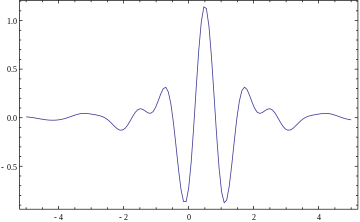
with the (normalized) sinc function. That, Meyer's, and two other examples of mother wavelets are:
The subspace of scale a or frequency band [1/a, 2/a] is generated by the functions (sometimes called child wavelets)
where a is positive and defines the scale and b is any real number and defines the shift. The pair (a, b) defines a point in the right halfplane R+ × R.
The projection of a function x onto the subspace of scale a then has the form
with wavelet coefficients
For the analysis of the signal x, one can assemble the wavelet coefficients into a scaleogram of the signal.
Discrete wavelet transforms (discrete shift and scale parameters, continuous in time)
It is computationally impossible to analyze a signal using all wavelet coefficients, so one may wonder if it is sufficient to pick a discrete subset of the upper halfplane to be able to reconstruct a signal from the corresponding wavelet coefficients. One such system is the affine system for some real parameters a > 1, b > 0. The corresponding discrete subset of the halfplane consists of all the points (am, nb am) with m, n in Z. The corresponding child wavelets are now given as
A sufficient condition for the reconstruction of any signal x of finite energy by the formula
Multiresolution based discrete wavelet transforms (continuous in time)
D4 wavelet
In any discretised wavelet transform, there are only a finite number of wavelet coefficients for each bounded rectangular region in the upper halfplane. Still, each coefficient requires the evaluation of an integral. In special situations this numerical complexity can be avoided if the scaled and shifted wavelets form a multiresolution analysis. This means that there has to exist an auxiliary function, the father wavelet φ in L2(R), and that a is an integer. A typical choice is a = 2 and b = 1. The most famous pair of father and mother wavelets is the Daubechies 4-tap wavelet. Note that not every orthonormal discrete wavelet basis can be associated to a multiresolution analysis; for example, the Journe wavelet admits no multiresolution analysis.[7]
From the mother and father wavelets one constructs the subspaces
The father wavelet keeps the time domain properties, while the mother wavelets keeps the frequency domain properties.
From these it is required that the sequence
forms a multiresolution analysis of L2 and that the subspaces are the orthogonal "differences" of the above sequence, that is, Wm is the orthogonal complement of Vm inside the subspace Vm−1,
In analogy to the sampling theorem one may conclude that the space Vm with sampling distance 2m more or less covers the frequency baseband from 0 to 1/2m-1. As orthogonal complement, Wm roughly covers the band [1/2m−1, 1/2m].
From those inclusions and orthogonality relations, especially , follows the existence of sequences and that satisfy the identities
so that and
so that
The second identity of the first pair is a refinement equation for the father wavelet φ. Both pairs of identities form the basis for the algorithm of the fast wavelet transform.
From the multiresolution analysis derives the orthogonal decomposition of the space L2 as
For any signal or function this gives a representation in basis functions of the corresponding subspaces as
where the coefficients are
and
Time-causal wavelets
For processing temporal signals in real time, it is essential that the wavelet filters do not access signal values from the future as well as that minimal temporal latencies can be obtained. Time-causal wavelets representations have been developed by Szu et al [8] and Lindeberg,[9] with the latter method also involving a memory-efficient time-recursive implementation.
Mother wavelet
For practical applications, and for efficiency reasons, one prefers continuously differentiable functions with compact support as mother (prototype) wavelet (functions). However, to satisfy analytical requirements (in the continuous WT) and in general for theoretical reasons, one chooses the wavelet functions from a subspace of the space This is the space of Lebesgue measurable functions that are both absolutely integrable and square integrable in the sense that
and
Being in this space ensures that one can formulate the conditions of zero mean and square norm one:
is the condition for zero mean, and
is the condition for square norm one.
For ψ to be a wavelet for the continuous wavelet transform (see there for exact statement), the mother wavelet must satisfy an admissibility criterion (loosely speaking, a kind of half-differentiability) in order to get a stably invertible transform.
For the discrete wavelet transform, one needs at least the condition that the wavelet series is a representation of the identity in the spaceL2(R). Most constructions of discrete WT make use of the multiresolution analysis, which defines the wavelet by a scaling function. This scaling function itself is a solution to a functional equation.
In most situations it is useful to restrict ψ to be a continuous function with a higher number M of vanishing moments, i.e. for all integer m < M
The mother wavelet is scaled (or dilated) by a factor of a and translated (or shifted) by a factor of b to give (under Morlet's original formulation):
For the continuous WT, the pair (a,b) varies over the full half-plane R+ × R; for the discrete WT this pair varies over a discrete subset of it, which is also called affine group.
These functions are often incorrectly referred to as the basis functions of the (continuous) transform. In fact, as in the continuous Fourier transform, there is no basis in the continuous wavelet transform. Time-frequency interpretation uses a subtly different formulation (after Delprat).
Restriction:
when a1 = a and b1 = b,
has a finite time interval
Comparisons with Fourier transform (continuous-time)
The wavelet transform is often compared with the Fourier transform, in which signals are represented as a sum of sinusoids. In fact, the Fourier transform can be viewed as a special case of the continuous wavelet transform with the choice of the mother wavelet . The main difference in general is that wavelets are localized in both time and frequency whereas the standard Fourier transform is only localized in frequency. The Short-time Fourier transform (STFT) is similar to the wavelet transform, in that it is also time and frequency localized, but there are issues with the frequency/time resolution trade-off.
In particular, assuming a rectangular window region, one may think of the STFT as a transform with a slightly different kernel
where can often be written as , where and u respectively denote the length and temporal offset of the windowing function. Using Parseval's theorem, one may define the wavelet's energy as
From this, the square of the temporal support of the window offset by time u is given by
and the square of the spectral support of the window acting on a frequency
Multiplication with a rectangular window in the time domain corresponds to convolution with a function in the frequency domain, resulting in spurious ringing artifacts for short/localized temporal windows. With the continuous-time Fourier Transform, and this convolution is with a delta function in Fourier space, resulting in the true Fourier transform of the signal . The window function may be some other apodizing filter, such as a Gaussian. The choice of windowing function will affect the approximation error relative to the true Fourier transform.
A given resolution cell's time-bandwidth product may not be exceeded with the STFT. All STFT basis elements maintain a uniform spectral and temporal support for all temporal shifts or offsets, thereby attaining an equal resolution in time for lower and higher frequencies. The resolution is purely determined by the sampling width.
In contrast, the wavelet transform's multiresolutional properties enables large temporal supports for lower frequencies while maintaining short temporal widths for higher frequencies by the scaling properties of the wavelet transform. This property extends conventional time-frequency analysis into time-scale analysis.[10]
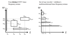
STFT time-frequency atoms (left) and DWT time-scale atoms (right). The time-frequency atoms are four different basis functions used for the STFT (i.e. four separate Fourier transforms required). The time-scale atoms of the DWT achieve small temporal widths for high frequencies and good temporal widths for low frequencies with a single transform basis set.
The discrete wavelet transform is less computationally complex, taking O(N) time as compared to O(NlogN) for the fast Fourier transform. This computational advantage is not inherent to the transform, but reflects the choice of a logarithmic division of frequency, in contrast to the equally spaced frequency divisions of the FFT (fast Fourier transform) which uses the same basis functions as DFT (Discrete Fourier Transform).[11] It is also important to note that this complexity only applies when the filter size has no relation to the signal size. A wavelet without compact support such as the Shannon wavelet would require O(N2). (For instance, a logarithmic Fourier Transform also exists with O(N) complexity, but the original signal must be sampled logarithmically in time, which is only useful for certain types of signals.[12])
Definition of a wavelet
A wavelet (or a wavelet family) can be defined in various ways:
Scaling filter
An orthogonal wavelet is entirely defined by the scaling filter – a low-pass finite impulse response (FIR) filter of length 2N and sum 1. In biorthogonal wavelets, separate decomposition and reconstruction filters are defined.
For analysis with orthogonal wavelets the high pass filter is calculated as the quadrature mirror filter of the low pass, and reconstruction filters are the time reverse of the decomposition filters.
Daubechies and Symlet wavelets can be defined by the scaling filter.
Scaling function
Wavelets are defined by the wavelet function ψ(t) (i.e. the mother wavelet) and scaling function φ(t) (also called father wavelet) in the time domain.
The wavelet function is in effect a band-pass filter and scaling that for each level halves its bandwidth. This creates the problem that in order to cover the entire spectrum, an infinite number of levels would be required. The scaling function filters the lowest level of the transform and ensures all the spectrum is covered. See[13] for a detailed explanation.
For a wavelet with compact support, φ(t) can be considered finite in length and is equivalent to the scaling filter g.
Meyer wavelets can be defined by scaling functions
Wavelet function
The wavelet only has a time domain representation as the wavelet function ψ(t).
The development of wavelets can be linked to several separate trains of thought, starting with Haar's work in the early 20th century. Later work by Dennis Gabor yielded Gabor atoms (1946), which are constructed similarly to wavelets, and applied to similar purposes.
Notable contributions to wavelet theory since then can be attributed to Zweig’s discovery of the continuous wavelet transform (CWT) in 1975 (originally called the cochlear transform and discovered while studying the reaction of the ear to sound),[14] Pierre Goupillaud, Grossmann and Morlet's formulation of what is now known as the CWT (1982), Jan-Olov Strömberg's early work on discrete wavelets (1983), the Le Gall–Tabatabai (LGT) 5/3-taps non-orthogonal filter bank with linear phase (1988),[15][16][17]Ingrid Daubechies' orthogonal wavelets with compact support (1988), Mallat's non-orthogonal multiresolution framework (1989), Ali Akansu's Binomial QMF (1990), Nathalie Delprat's time-frequency interpretation of the CWT (1991), Newland's harmonic wavelet transform (1993), and set partitioning in hierarchical trees (SPIHT) developed by Amir Said with William A. Pearlman in 1996.[18]
A wavelet is a mathematical function used to divide a given function or continuous-time signal into different scale components. Usually one can assign a frequency range to each scale component. Each scale component can then be studied with a resolution that matches its scale. A wavelet transform is the representation of a function by wavelets. The wavelets are scaled and translated copies (known as "daughter wavelets") of a finite-length or fast-decaying oscillating waveform (known as the "mother wavelet"). Wavelet transforms have advantages over traditional Fourier transforms for representing functions that have discontinuities and sharp peaks, and for accurately deconstructing and reconstructing finite, non-periodic and/or non-stationary signals.
Wavelet transforms are classified into discrete wavelet transforms (DWTs) and continuous wavelet transforms (CWTs). Note that both DWT and CWT are continuous-time (analog) transforms. They can be used to represent continuous-time (analog) signals. CWTs operate over every possible scale and translation whereas DWTs use a specific subset of scale and translation values or representation grid.
There are a large number of wavelet transforms each suitable for different applications. For a full list see list of wavelet-related transforms but the common ones are listed below:
There are a number of generalized transforms of which the wavelet transform is a special case. For example, Yosef Joseph Segman introduced scale into the Heisenberg group, giving rise to a continuous transform space that is a function of time, scale, and frequency. The CWT is a two-dimensional slice through the resulting 3d time-scale-frequency volume.
Another example of a generalized transform is the chirplet transform in which the CWT is also a two dimensional slice through the chirplet transform.
An important application area for generalized transforms involves systems in which high frequency resolution is crucial. For example, darkfield electron optical transforms intermediate between direct and reciprocal space have been widely used in the harmonic analysis of atom clustering, i.e. in the study of crystals and crystal defects.[22] Now that transmission electron microscopes are capable of providing digital images with picometer-scale information on atomic periodicity in nanostructure of all sorts, the range of pattern recognition[23] and strain[24]/metrology[25] applications for intermediate transforms with high frequency resolution (like brushlets[26] and ridgelets[27]) is growing rapidly.
Fractional wavelet transform (FRWT) is a generalization of the classical wavelet transform in the fractional Fourier transform domains. This transform is capable of providing the time- and fractional-domain information simultaneously and representing signals in the time-fractional-frequency plane.[28]
Applications
Generally, an approximation to DWT is used for data compression if a signal is already sampled, and the CWT for signal analysis.[29] Thus, DWT approximation is commonly used in engineering and computer science,[30] and the CWT in scientific research.[31]
Like some other transforms, wavelet transforms can be used to transform data, then encode the transformed data, resulting in effective compression. For example, JPEG 2000 is an image compression standard that uses biorthogonal wavelets. This means that although the frame is overcomplete, it is a tight frame (see types of frames of a vector space), and the same frame functions (except for conjugation in the case of complex wavelets) are used for both analysis and synthesis, i.e., in both the forward and inverse transform. For details see wavelet compression.
A related use is for smoothing/denoising data based on wavelet coefficient thresholding, also called wavelet shrinkage. By adaptively thresholding the wavelet coefficients that correspond to undesired frequency components smoothing and/or denoising operations can be performed.
Wavelet transforms are also starting to be used for communication applications. Wavelet OFDM is the basic modulation scheme used in HD-PLC (a power line communications technology developed by Panasonic), and in one of the optional modes included in the IEEE 1901 standard. Wavelet OFDM can achieve deeper notches than traditional FFT OFDM, and wavelet OFDM does not require a guard interval (which usually represents significant overhead in FFT OFDM systems).[32]
As a representation of a signal
Often, signals can be represented well as a sum of sinusoids. However, consider a non-continuous signal with an abrupt discontinuity; this signal can still be represented as a sum of sinusoids, but requires an infinite number, which is an observation known as Gibbs phenomenon. This, then, requires an infinite number of Fourier coefficients, which is not practical for many applications, such as compression. Wavelets are more useful for describing these signals with discontinuities because of their time-localized behavior (both Fourier and wavelet transforms are frequency-localized, but wavelets have an additional time-localization property). Because of this, many types of signals in practice may be non-sparse in the Fourier domain, but very sparse in the wavelet domain. This is particularly useful in signal reconstruction, especially in the recently popular field of compressed sensing. (Note that the short-time Fourier transform (STFT) is also localized in time and frequency, but there are often problems with the frequency-time resolution trade-off. Wavelets are better signal representations because of multiresolution analysis.)
Signal denoising by wavelet transform thresholding
Suppose we measure a noisy signal , where represents the signal and represents the noise. Assume has a sparse representation in a certain wavelet basis, and
Let the wavelet transform of be , where is the wavelet transform of the signal component and is the wavelet transform of the noise component.
Most elements in are 0 or close to 0, and
Since is orthogonal, the estimation problem amounts to recovery of a signal in iid Gaussian noise. As is sparse, one method is to apply a Gaussian mixture model for .
Assume a prior , where is the variance of "significant" coefficients and is the variance of "insignificant" coefficients.
Then , is called the shrinkage factor, which depends on the prior variances and . By setting coefficients that fall below a shrinkage threshold to zero, once the inverse transform is applied, an expectedly small amount of signal is lost due to the sparsity assumption. The larger coefficients are expected to primarily represent signal due to sparsity, and statistically very little of the signal, albeit the majority of the noise, is expected to be represented in such lower magnitude coefficients... therefore the zeroing-out operation is expected to remove most of the noise and not much signal. Typically, the above-threshold coefficients are not modified during this process. Some algorithms for wavelet-based denoising may attenuate larger coefficients as well, based on a statistical estimate of the amount of noise expected to be removed by such an attenuation.
At last, apply the inverse wavelet transform to obtain
Multiscale climate network
Agarwal et al. proposed wavelet based advanced linear [39] and nonlinear [40] methods to construct and investigate Climate as complex networks at different timescales. Climate networks constructed using SST datasets at different timescale averred that wavelet based multi-scale analysis of climatic processes holds the promise of better understanding the system dynamics that may be missed when processes are analyzed at one timescale only [41]
In mathematics, Fourier analysis is the study of the way general functions may be represented or approximated by sums of simpler trigonometric functions. Fourier analysis grew from the study of Fourier series, and is named after Joseph Fourier, who showed that representing a function as a sum of trigonometric functions greatly simplifies the study of heat transfer.
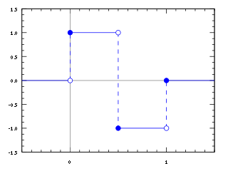
In mathematics, the Haar wavelet is a sequence of rescaled "square-shaped" functions which together form a wavelet family or basis. Wavelet analysis is similar to Fourier analysis in that it allows a target function over an interval to be represented in terms of an orthonormal basis. The Haar sequence is now recognised as the first known wavelet basis and is extensively used as a teaching example.
The Daubechies wavelets, based on the work of Ingrid Daubechies, are a family of orthogonal wavelets defining a discrete wavelet transform and characterized by a maximal number of vanishing moments for some given support. With each wavelet type of this class, there is a scaling function which generates an orthogonal multiresolution analysis.
In mathematics, the continuous wavelet transform (CWT) is a formal tool that provides an overcomplete representation of a signal by letting the translation and scale parameter of the wavelets vary continuously.
In numerical analysis and functional analysis, a discrete wavelet transform (DWT) is any wavelet transform for which the wavelets are discretely sampled. As with other wavelet transforms, a key advantage it has over Fourier transforms is temporal resolution: it captures both frequency and location information.
Stransform as a time–frequency distribution was developed in 1994 for analyzing geophysics data. In this way, the S transform is a generalization of the short-time Fourier transform (STFT), extending the continuous wavelet transform and overcoming some of its disadvantages. For one, modulation sinusoids are fixed with respect to the time axis; this localizes the scalable Gaussian window dilations and translations in S transform. Moreover, the S transform doesn't have a cross-term problem and yields a better signal clarity than Gabor transform. However, the S transform has its own disadvantages: the clarity is worse than Wigner distribution function and Cohen's class distribution function.
The fast wavelet transform is a mathematical algorithm designed to turn a waveform or signal in the time domain into a sequence of coefficients based on an orthogonal basis of small finite waves, or wavelets. The transform can be easily extended to multidimensional signals, such as images, where the time domain is replaced with the space domain. This algorithm was introduced in 1989 by Stéphane Mallat.
Coiflets are discrete wavelets designed by Ingrid Daubechies, at the request of Ronald Coifman, to have scaling functions with vanishing moments. The wavelet is near symmetric, their wavelet functions have vanishing moments and scaling functions , and has been used in many applications using Calderón–Zygmund operators.
A multiresolution analysis (MRA) or multiscale approximation (MSA) is the design method of most of the practically relevant discrete wavelet transforms (DWT) and the justification for the algorithm of the fast wavelet transform (FWT). It was introduced in this context in 1988/89 by Stephane Mallat and Yves Meyer and has predecessors in the microlocal analysis in the theory of differential equations and the pyramid methods of image processing as introduced in 1981/83 by Peter J. Burt, Edward H. Adelson and James L. Crowley.
Originally known as optimal subband tree structuring (SB-TS), also called wavelet packet decomposition, is a wavelet transform where the discrete-time (sampled) signal is passed through more filters than the discrete wavelet transform (DWT).
In mathematics, a wavelet series is a representation of a square-integrable function by a certain orthonormal series generated by a wavelet. This article provides a formal, mathematical definition of an orthonormal wavelet and of the integral wavelet transform.
The Gabor transform, named after Dennis Gabor, is a special case of the short-time Fourier transform. It is used to determine the sinusoidal frequency and phase content of local sections of a signal as it changes over time. The function to be transformed is first multiplied by a Gaussian function, which can be regarded as a window function, and the resulting function is then transformed with a Fourier transform to derive the time-frequency analysis. The window function means that the signal near the time being analyzed will have higher weight. The Gabor transform of a signal x(t) is defined by this formula:
Geophysical survey is the systematic collection of geophysical data for spatial studies. Detection and analysis of the geophysical signals forms the core of Geophysical signal processing. The magnetic and gravitational fields emanating from the Earth's interior hold essential information concerning seismic activities and the internal structure. Hence, detection and analysis of the electric and Magnetic fields is very crucial. As the Electromagnetic and gravitational waves are multi-dimensional signals, all the 1-D transformation techniques can be extended for the analysis of these signals as well. Hence this article also discusses multi-dimensional signal processing techniques.
Continuous wavelets of compact support alpha can be built, which are related to the beta distribution. The process is derived from probability distributions using blur derivative. These new wavelets have just one cycle, so they are termed unicycle wavelets. They can be viewed as a soft variety of Haar wavelets whose shape is fine-tuned by two parameters and . Closed-form expressions for beta wavelets and scale functions as well as their spectra are derived. Their importance is due to the Central Limit Theorem by Gnedenko and Kolmogorov applied for compactly supported signals.
In functional analysis, the Shannon wavelet is a decomposition that is defined by signal analysis by ideal bandpass filters. Shannon wavelet may be either of real or complex type.
The Mathieu equation is a linear second-order differential equation with periodic coefficients. The French mathematician, E. Léonard Mathieu, first introduced this family of differential equations, nowadays termed Mathieu equations, in his “Memoir on vibrations of an elliptic membrane” in 1868. "Mathieu functions are applicable to a wide variety of physical phenomena, e.g., diffraction, amplitude distortion, inverted pendulum, stability of a floating body, radio frequency quadrupole, and vibration in a medium with modulated density"
Fractional wavelet transform (FRWT) is a generalization of the classical wavelet transform (WT). This transform is proposed in order to rectify the limitations of the WT and the fractional Fourier transform (FRFT). The FRWT inherits the advantages of multiresolution analysis of the WT and has the capability of signal representations in the fractional domain which is similar to the FRFT.
In applied mathematical analysis, shearlets are a multiscale framework which allows efficient encoding of anisotropic features in multivariate problem classes. Originally, shearlets were introduced in 2006 for the analysis and sparse approximation of functions . They are a natural extension of wavelets, to accommodate the fact that multivariate functions are typically governed by anisotropic features such as edges in images, since wavelets, as isotropic objects, are not capable of capturing such phenomena.
In mathematics, in functional analysis, several different wavelets are known by the name Poisson wavelet. In one context, the term "Poisson wavelet" is used to denote a family of wavelets labeled by the set of positive integers, the members of which are associated with the Poisson probability distribution. These wavelets were first defined and studied by Karlene A. Kosanovich, Allan R. Moser and Michael J. Piovoso in 1995–96. In another context, the term refers to a certain wavelet which involves a form of the Poisson integral kernel. In still another context, the terminology is used to describe a family of complex wavelets indexed by positive integers which are connected with the derivatives of the Poisson integral kernel.
Multiresolution Fourier Transform is an integral fourier transform that represents a specific wavelet-like transform with a fully scalable modulated window, but not all possible translations.
References
↑ Wireless Communications: Principles and Practice, Prentice Hall communications engineering and emerging technologies series, T.S. Rappaport, Prentice Hall, 2002, p.126.
↑ Akansu, Ali N.; Haddad, Richard A. (1992), Multiresolution Signal Decomposition: Transforms, Subbands, and Wavelets, Boston, MA: Academic Press, ISBN978-0-12-047141-6
↑ Larson, David R. (2007), Wavelet Analysis and Applications (See: Unitary systems and wavelet sets), Appl. Numer. Harmon. Anal., Birkhäuser, pp.143–171
↑ Gall, Didier Le; Tabatabai, Ali J. (1988). "Sub-band coding of digital images using symmetric short kernel filters and arithmetic coding techniques". ICASSP-88., International Conference on Acoustics, Speech, and Signal Processing. pp.761–764 vol.2. doi:10.1109/ICASSP.1988.196696. S2CID109186495.
↑ Said, Amir; Pearlman, William A. (June 1996). "A new fast and efficient image codec based on set partitioning in hierarchical trees". IEEE Transactions on Circuits and Systems for Video Technology. 6 (3): 243–250. doi:10.1109/76.499834. ISSN1051-8215.
↑ P. Hirsch, A. Howie, R. Nicholson, D. W. Pashley and M. J. Whelan (1965/1977) Electron microscopy of thin crystals (Butterworths, London/Krieger, Malabar FLA) ISBN0-88275-376-2
↑ P. Fraundorf, J. Wang, E. Mandell and M. Rose (2006) Digital darkfield tableaus, Microscopy and Microanalysis12:S2, 1010–1011 (cf. arXiv:cond-mat/0403017)
↑ Hÿtch, M. J.; Snoeck, E.; Kilaas, R. (1998). "Quantitative measurement of displacement and strain fields from HRTEM micrographs". Ultramicroscopy. 74 (3): 131–146. doi:10.1016/s0304-3991(98)00035-7.
↑ Martin Rose (2006) Spacing measurements of lattice fringes in HRTEM image using digital darkfield decomposition (M.S. Thesis in Physics, U. Missouri – St. Louis)
↑ A. G. Flesia, H. Hel-Or, A. Averbuch, E. J. Candes, R. R. Coifman and D. L. Donoho (2001) Digital implementation of ridgelet packets (Academic Press, New York).
↑ Shi, J.; Zhang, N.-T.; Liu, X.-P. (2011). "A novel fractional wavelet transform and its applications". Sci. China Inf. Sci. 55 (6): 1270–1279. doi:10.1007/s11432-011-4320-x. S2CID255201598.
↑ Lyakhov, Pavel; Semyonova, Nataliya; Nagornov, Nikolay; Bergerman, Maxim; Abdulsalyamova, Albina (2023-11-14). "High-Speed Wavelet Image Processing Using the Winograd Method with Downsampling". Mathematics. 11 (22): 4644. doi:10.3390/math11224644. ISSN2227-7390. Wavelets are actively used to solve a wide range of image processing problems in various fields of science and technology, e.g., image denoising, reconstruction, analysis, and video analysis and processing. Wavelet processing methods are based on the discrete wavelet transform using 1D digital filtering.
↑ Stefano Galli; O. Logvinov (July 2008). "Recent Developments in the Standardization of Power Line Communications within the IEEE". IEEE Communications Magazine. 46 (7): 64–71. doi:10.1109/MCOM.2008.4557044. S2CID2650873. An overview of P1901 PHY/MAC proposal.
Donald B. Percival and Andrew T. Walden, Wavelet Methods for Time Series Analysis, Cambridge University Press, 2000, ISBN0-521-68508-7.
Ramazan Gençay, Faruk Selçuk and Brandon Whitcher, An Introduction to Wavelets and Other Filtering Methods in Finance and Economics, Academic Press, 2001, ISBN0-12-279670-5.
Press, W. H.; Teukolsky, S. A.; Vetterling, W. T.; Flannery, B. P. (2007), "Section 13.10. Wavelet Transforms", Numerical Recipes: The Art of Scientific Computing (3rded.), New York: Cambridge University Press, ISBN978-0-521-88068-8, archived from the original on 2011-08-11, retrieved 2011-08-13.
WITS: Where Is The Starlet? A dictionary of tens of wavelets and wavelet-related terms ending in -let, from activelets to x-lets through bandlets, contourlets, curvelets, noiselets, wedgelets.
This page is based on this Wikipedia article Text is available under the CC BY-SA 4.0 license; additional terms may apply. Images, videos and audio are available under their respective licenses.