Definition
Let the lifetime T be a continuous random variable with cumulative hazard function F(t) and hazard function f(t) on the interval [0,∞). Its survival function or reliability function is:
The survival function is a function that gives the probability that a patient, device, or other object of interest will survive past a certain time. [1] The survival function is also known as the survivor function [2] or reliability function. [3] The term reliability function is common in engineering while the term survival function is used in a broader range of applications, including human mortality. The survival function is the complementary cumulative distribution function of the lifetime. Sometimes complementary cumulative distribution functions are called survival functions in general.
Let the lifetime T be a continuous random variable with cumulative hazard function F(t) and hazard function f(t) on the interval [0,∞). Its survival function or reliability function is:
The graphs below show examples of hypothetical survival functions. The x-axis is time. The y-axis is the proportion of subjects surviving. The graphs show the probability that a subject will survive beyond time t.
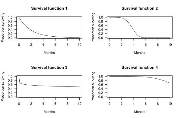
For example, for survival function 1, the probability of surviving longer than t = 2 months is 0.37. That is, 37% of subjects survive more than 2 months.

For survival function 2, the probability of surviving longer than t = 2 months is 0.97. That is, 97% of subjects survive more than 2 months.

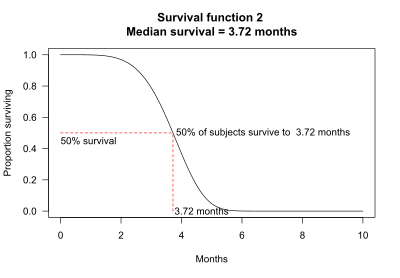
Median survival may be determined from the survival function: The median survival is the point where the survival function intersects the value 0.5. [4] For example, for survival function 2, 50% of the subjects survive 3.72 months. Median survival is thus 3.72 months.
In some cases, median survival cannot be determined from the graph. For example, for survival function 4, more than 50% of the subjects survive longer than the observation period of 10 months.

The survival function is one of several ways to describe and display survival data. Another useful way to display data is a graph showing the distribution of survival times of subjects. Olkin, [5] page 426, gives the following example of survival data. The number of hours between successive failures of an air-conditioning system were recorded. The time between successive failures are 1, 3, 5, 7, 11, 11, 11, 12, 14, 14, 14, 16, 16, 20, 21, 23, 42, 47, 52, 62, 71, 71, 87, 90, 95, 120, 120, 225, 246, and 261 hours. The mean time between failures is 59.6. This mean value will be used shortly to fit a theoretical curve to the data. The figure below shows the distribution of the time between failures. The blue tick marks beneath the graph are the actual hours between successive failures.
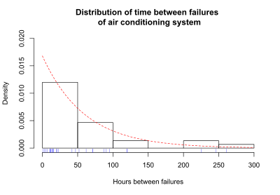
The distribution of failure times is over-laid with a curve representing an exponential distribution. For this example, the exponential distribution approximates the distribution of failure times. The exponential curve is a theoretical distribution fitted to the actual failure times. This particular exponential curve is specified by the parameter lambda, λ= 1/(mean time between failures) = 1/59.6 = 0.0168. The distribution of failure times is called the probability density function (pdf), if time can take any positive value. In equations, the pdf is specified as f(t). If time can only take discrete values (such as 1 day, 2 days, and so on), the distribution of failure times is called the probability mass function (pmf). Most survival analysis methods assume that time can take any positive value, and f(t) is the pdf. If the time between observed air conditioner failures is approximated using the exponential function, then the exponential curve gives the probability density function, f(t), for air conditioner failure times.
Another useful way to display the survival data is a graph showing the cumulative failures up to each time point. These data may be displayed as either the cumulative number or the cumulative proportion of failures up to each time. The graph below shows the cumulative probability (or proportion) of failures at each time for the air conditioning system. The stairstep line in black shows the cumulative proportion of failures. For each step there is a blue tick at the bottom of the graph indicating an observed failure time. The smooth red line represents the exponential curve fitted to the observed data.
A graph of the cumulative probability of failures up to each time point is called the cumulative distribution function, or CDF. In survival analysis, the cumulative distribution function gives the probability that the survival time is less than or equal to a specific time, t.
Let T be survival time, which is any positive number. A particular time is designated by the lower case letter t. The cumulative distribution function of T is the function
where the right-hand side represents the probability that the random variable T is less than or equal to t. If time can take on any positive value, then the cumulative distribution function F(t) is the integral of the probability density function f(t).
For the air conditioning example, the graph of the CDF below illustrates that the probability that the time to failure is less than or equal to 100 hours is 0.81, as estimated using the exponential curve fit to the data.
An alternative to graphing the probability that the failure time is less than or equal to 100 hours is to graph the probability that the failure time is greater than 100 hours. The probability that the failure time is greater than 100 hours must be 1 minus the probability that the failure time is less than or equal to 100 hours, because total probability must sum to 1.
This gives
P(failure time > 100 hours) = 1 - P(failure time < 100 hours) = 1 – 0.81 = 0.19.
This relationship generalizes to all failure times:
P(T > t) = 1 - P(T < t) = 1 – cumulative distribution function.
This relationship is shown on the graphs below. The graph on the left is the cumulative distribution function, which is P(T < t). The graph on the right is P(T > t) = 1 - P(T < t). The graph on the right is the survival function, S(t). The fact that the S(t) = 1 – CDF is the reason that another name for the survival function is the complementary cumulative distribution function.
In some cases, such as the air conditioner example, the distribution of survival times may be approximated well by a function such as the exponential distribution. Several distributions are commonly used in survival analysis, including the exponential, Weibull, gamma, normal, log-normal, and log-logistic. [3] [6] These distributions are defined by parameters. The normal (Gaussian) distribution, for example, is defined by the two parameters mean and standard deviation. Survival functions that are defined by parameters are said to be parametric.
In the four survival function graphs shown above, the shape of the survival function is defined by a particular probability distribution: survival function 1 is defined by an exponential distribution, 2 is defined by a Weibull distribution, 3 is defined by a log-logistic distribution, and 4 is defined by another Weibull distribution.
For an exponential survival distribution, the probability of failure is the same in every time interval, no matter the age of the individual or device. This fact leads to the "memoryless" property of the exponential survival distribution: the age of a subject has no effect on the probability of failure in the next time interval. The exponential may be a good model for the lifetime of a system where parts are replaced as they fail. [7] It may also be useful for modeling survival of living organisms over short intervals. It is not likely to be a good model of the complete lifespan of a living organism. [8] As Efron and Hastie [9] (p. 134) note, "If human lifetimes were exponential there wouldn't be old or young people, just lucky or unlucky ones".
A key assumption of the exponential survival function is that the hazard rate is constant. In an example given above, the proportion of men dying each year was constant at 10%, meaning that the hazard rate was constant. The assumption of constant hazard may not be appropriate. For example, among most living organisms, the risk of death is greater in old age than in middle age – that is, the hazard rate increases with time. For some diseases, such as breast cancer, the risk of recurrence is lower after 5 years – that is, the hazard rate decreases with time. The Weibull distribution extends the exponential distribution to allow constant, increasing, or decreasing hazard rates.
There are several other parametric survival functions that may provide a better fit to a particular data set, including normal, lognormal, log-logistic, and gamma. The choice of parametric distribution for a particular application can be made using graphical methods or using formal tests of fit. These distributions and tests are described in textbooks on survival analysis. [1] [3] Lawless [10] has extensive coverage of parametric models.
Parametric survival functions are commonly used in manufacturing applications, in part because they enable estimation of the survival function beyond the observation period. However, appropriate use of parametric functions requires that data are well modeled by the chosen distribution. If an appropriate distribution is not available, or cannot be specified before a clinical trial or experiment, then non-parametric survival functions offer a useful alternative.
A parametric model of survival may not be possible or desirable. In these situations, the most common method to model the survival function is the non-parametric Kaplan–Meier estimator. This estimator requires lifetime data. Periodic case (cohort) and death (and recovery) counts are statistically sufficient to make non-parametric maximum likelihood and least squares estimates of survival functions, without lifetime data.
So that
Proof of expected survival time formula |
|---|
| The expected value of a random variable is defined as: where is the probability density function. Using the relation , the expected value formula may be modified: This may be further simplified by employing integration by parts: By definition, , meaning that the boundary terms are identically equal to zero. Therefore, we may conclude that the expected value is simply the integral of the survival function: |

In probability theory and statistics, the exponential distribution or negative exponential distribution is the probability distribution of the time between events in a Poisson point process, i.e., a process in which events occur continuously and independently at a constant average rate. It is a particular case of the gamma distribution. It is the continuous analogue of the geometric distribution, and it has the key property of being memoryless. In addition to being used for the analysis of Poisson point processes it is found in various other contexts.
Mean time between failures (MTBF) is the predicted elapsed time between inherent failures of a mechanical or electronic system during normal system operation. MTBF can be calculated as the arithmetic mean (average) time between failures of a system. The term is used for repairable systems while mean time to failure (MTTF) denotes the expected time to failure for a non-repairable system.

In probability theory and statistics, the Weibull distribution is a continuous probability distribution. It models a broad range of random variables, largely in the nature of a time to failure or time between events. Examples are maximum one-day rainfalls and the time a user spends on a web page.
In survival analysis, the hazard ratio (HR) is the ratio of the hazard rates corresponding to the conditions characterised by two distinct levels of a treatment variable of interest. For example, in a clinical study of a drug, the treated population may die at twice the rate per unit time of the control population. The hazard ratio would be 2, indicating a higher hazard of death from the treatment.
Survival analysis is a branch of statistics for analyzing the expected duration of time until one event occurs, such as death in biological organisms and failure in mechanical systems. This topic is called reliability theory or reliability analysis in engineering, duration analysis or duration modelling in economics, and event history analysis in sociology. Survival analysis attempts to answer certain questions, such as what is the proportion of a population which will survive past a certain time? Of those that survive, at what rate will they die or fail? Can multiple causes of death or failure be taken into account? How do particular circumstances or characteristics increase or decrease the probability of survival?
Failure rate is the frequency with which an engineered system or component fails, expressed in failures per unit of time. It is usually denoted by the Greek letter λ (lambda) and is often used in reliability engineering.
In convex analysis, a non-negative function f : Rn → R+ is logarithmically concave if its domain is a convex set, and if it satisfies the inequality
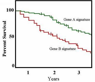
The Kaplan–Meier estimator, also known as the product limit estimator, is a non-parametric statistic used to estimate the survival function from lifetime data. In medical research, it is often used to measure the fraction of patients living for a certain amount of time after treatment. In other fields, Kaplan–Meier estimators may be used to measure the length of time people remain unemployed after a job loss, the time-to-failure of machine parts, or how long fleshy fruits remain on plants before they are removed by frugivores. The estimator is named after Edward L. Kaplan and Paul Meier, who each submitted similar manuscripts to the Journal of the American Statistical Association. The journal editor, John Tukey, convinced them to combine their work into one paper, which has been cited more than 61,800 times since its publication in 1958.
In statistics, censoring is a condition in which the value of a measurement or observation is only partially known.

In probability and statistics, the log-logistic distribution is a continuous probability distribution for a non-negative random variable. It is used in survival analysis as a parametric model for events whose rate increases initially and decreases later, as, for example, mortality rate from cancer following diagnosis or treatment. It has also been used in hydrology to model stream flow and precipitation, in economics as a simple model of the distribution of wealth or income, and in networking to model the transmission times of data considering both the network and the software.
In the statistical area of survival analysis, an accelerated failure time model is a parametric model that provides an alternative to the commonly used proportional hazards models. Whereas a proportional hazards model assumes that the effect of a covariate is to multiply the hazard by some constant, an AFT model assumes that the effect of a covariate is to accelerate or decelerate the life course of a disease by some constant. This is especially appealing in a technical context where the 'disease' is a result of some mechanical process with a known sequence of intermediary stages.
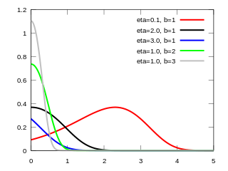
In probability and statistics, the Gompertz distribution is a continuous probability distribution, named after Benjamin Gompertz. The Gompertz distribution is often applied to describe the distribution of adult lifespans by demographers and actuaries. Related fields of science such as biology and gerontology also considered the Gompertz distribution for the analysis of survival. More recently, computer scientists have also started to model the failure rates of computer code by the Gompertz distribution. In Marketing Science, it has been used as an individual-level simulation for customer lifetime value modeling. In network theory, particularly the Erdős–Rényi model, the walk length of a random self-avoiding walk (SAW) is distributed according to the Gompertz distribution.

In probability theory and statistics, the Exponential-Logarithmic (EL) distribution is a family of lifetime distributions with decreasing failure rate, defined on the interval [0, ∞). This distribution is parameterized by two parameters and .

The generalized gamma distribution is a continuous probability distribution with two shape parameters. It is a generalization of the gamma distribution which has one shape parameter. Since many distributions commonly used for parametric models in survival analysis are special cases of the generalized gamma, it is sometimes used to determine which parametric model is appropriate for a given set of data. Another example is the half-normal distribution.
In statistics, the exponentiated Weibull family of probability distributions was introduced by Mudholkar and Srivastava (1993) as an extension of the Weibull family obtained by adding a second shape parameter.
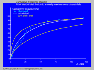
In statistics and data analysis the application software CumFreq is a tool for cumulative frequency analysis of a single variable and for probability distribution fitting.
Probability distribution fitting or simply distribution fitting is the fitting of a probability distribution to a series of data concerning the repeated measurement of a variable phenomenon. The aim of distribution fitting is to predict the probability or to forecast the frequency of occurrence of the magnitude of the phenomenon in a certain interval.
Hypertabastic survival models were introduced in 2007 by Mohammad Tabatabai, Zoran Bursac, David Williams, and Karan Singh. This distribution can be used to analyze time-to-event data in biomedical and public health areas and normally called survival analysis. In engineering, the time-to event analysis is referred to as reliability theory and in business and economics it is called duration analysis. Other fields may use different names for the same analysis. These survival models are applicable in many fields such as biomedical, behavioral science, social science, statistics, medicine, bioinformatics, medicalinformatics, data science especially in machine learning, computational biology, business economics, engineering, and commercial entities. They not only look at the time to event, but whether or not the event occurred. These time-to-event models can be applied in a variety of applications for instance, time after diagnosis of cancer until death, comparison of individualized treatment with standard care in cancer research, time until an individual defaults on loans, relapsed time for drug and smoking cessation, time until property sold after being put on the market, time until an individual upgrades to a new phone, time until job relocation, time until bones receive microscopic fractures when undergoing different stress levels, time from marriage until divorce, time until infection due to catheter, and time from bridge completion until first repair.

The Kaniadakis Weibull distribution is a probability distribution arising as a generalization of the Weibull distribution. It is one example of a Kaniadakis κ-distribution. The κ-Weibull distribution has been adopted successfully for describing a wide variety of complex systems in seismology, economy, epidemiology, among many others.

The Kaniadakis Logistic distribution is a generalized version of the Logistic distribution associated with the Kaniadakis statistics. It is one example of a Kaniadakis distribution. The κ-Logistic probability distribution describes the population kinetics behavior of bosonic or fermionic character.