
In statistics, a normal distribution or Gaussian distribution is a type of continuous probability distribution for a real-valued random variable. The general form of its probability density function is
In probability theory, the central limit theorem (CLT) states that, under appropriate conditions, the distribution of a normalized version of the sample mean converges to a standard normal distribution. This holds even if the original variables themselves are not normally distributed. There are several versions of the CLT, each applying in the context of different conditions.

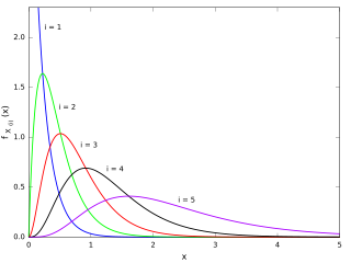
In probability theory and statistics, the chi-squared distribution with degrees of freedom is the distribution of a sum of the squares of independent standard normal random variables. The chi-squared distribution is a special case of the gamma distribution and is one of the most widely used probability distributions in inferential statistics, notably in hypothesis testing and in construction of confidence intervals. This distribution is sometimes called the central chi-squared distribution, a special case of the more general noncentral chi-squared distribution.
In statistics, maximum likelihood estimation (MLE) is a method of estimating the parameters of an assumed probability distribution, given some observed data. This is achieved by maximizing a likelihood function so that, under the assumed statistical model, the observed data is most probable. The point in the parameter space that maximizes the likelihood function is called the maximum likelihood estimate. The logic of maximum likelihood is both intuitive and flexible, and as such the method has become a dominant means of statistical inference.
In statistics, the kth order statistic of a statistical sample is equal to its kth-smallest value. Together with rank statistics, order statistics are among the most fundamental tools in non-parametric statistics and inference.
In mathematical analysis, asymptotic analysis, also known as asymptotics, is a method of describing limiting behavior.
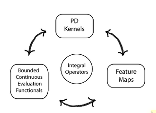
In functional analysis, a reproducing kernel Hilbert space (RKHS) is a Hilbert space of functions in which point evaluation is a continuous linear functional. Roughly speaking, this means that if two functions and in the RKHS are close in norm, i.e., is small, then and are also pointwise close, i.e., is small for all . The converse does not need to be true. Informally, this can be shown by looking at the supremum norm: the sequence of functions converges pointwise, but does not converge uniformly i.e. does not converge with respect to the supremum norm.
Directional statistics is the subdiscipline of statistics that deals with directions, axes or rotations in Rn. More generally, directional statistics deals with observations on compact Riemannian manifolds including the Stiefel manifold.
In probability and statistics, a circular distribution or polar distribution is a probability distribution of a random variable whose values are angles, usually taken to be in the range [0, 2π). A circular distribution is often a continuous probability distribution, and hence has a probability density, but such distributions can also be discrete, in which case they are called circular lattice distributions. Circular distributions can be used even when the variables concerned are not explicitly angles: the main consideration is that there is not usually any real distinction between events occurring at the lower or upper end of the range, and the division of the range could notionally be made at any point.

In probability theory and directional statistics, the von Mises distribution is a continuous probability distribution on the circle. It is a close approximation to the wrapped normal distribution, which is the circular analogue of the normal distribution. A freely diffusing angle on a circle is a wrapped normally distributed random variable with an unwrapped variance that grows linearly in time. On the other hand, the von Mises distribution is the stationary distribution of a drift and diffusion process on the circle in a harmonic potential, i.e. with a preferred orientation. The von Mises distribution is the maximum entropy distribution for circular data when the real and imaginary parts of the first circular moment are specified. The von Mises distribution is a special case of the von Mises–Fisher distribution on the N-dimensional sphere.

In statistics, kernel density estimation (KDE) is the application of kernel smoothing for probability density estimation, i.e., a non-parametric method to estimate the probability density function of a random variable based on kernels as weights. KDE answers a fundamental data smoothing problem where inferences about the population are made, based on a finite data sample. In some fields such as signal processing and econometrics it is also termed the Parzen–Rosenblatt window method, after Emanuel Parzen and Murray Rosenblatt, who are usually credited with independently creating it in its current form. One of the famous applications of kernel density estimation is in estimating the class-conditional marginal densities of data when using a naive Bayes classifier, which can improve its prediction accuracy.

In statistics, an empirical distribution function is the distribution function associated with the empirical measure of a sample. This cumulative distribution function is a step function that jumps up by 1/n at each of the n data points. Its value at any specified value of the measured variable is the fraction of observations of the measured variable that are less than or equal to the specified value.
The Anderson–Darling test is a statistical test of whether a given sample of data is drawn from a given probability distribution. In its basic form, the test assumes that there are no parameters to be estimated in the distribution being tested, in which case the test and its set of critical values is distribution-free. However, the test is most often used in contexts where a family of distributions is being tested, in which case the parameters of that family need to be estimated and account must be taken of this in adjusting either the test-statistic or its critical values. When applied to testing whether a normal distribution adequately describes a set of data, it is one of the most powerful statistical tools for detecting most departures from normality. K-sample Anderson–Darling tests are available for testing whether several collections of observations can be modelled as coming from a single population, where the distribution function does not have to be specified.
In statistics the Cramér–von Mises criterion is a criterion used for judging the goodness of fit of a cumulative distribution function compared to a given empirical distribution function , or for comparing two empirical distributions. It is also used as a part of other algorithms, such as minimum distance estimation. It is defined as
In probability theory, heavy-tailed distributions are probability distributions whose tails are not exponentially bounded: that is, they have heavier tails than the exponential distribution. In many applications it is the right tail of the distribution that is of interest, but a distribution may have a heavy left tail, or both tails may be heavy.
In statistics, kernel regression is a non-parametric technique to estimate the conditional expectation of a random variable. The objective is to find a non-linear relation between a pair of random variables X and Y.
In statistical theory, a U-statistic is a class of statistics defined as the average over the application of a given function applied to all tuples of a fixed size. The letter "U" stands for unbiased. In elementary statistics, U-statistics arise naturally in producing minimum-variance unbiased estimators.

In probability theory and directional statistics, a wrapped normal distribution is a wrapped probability distribution that results from the "wrapping" of the normal distribution around the unit circle. It finds application in the theory of Brownian motion and is a solution to the heat equation for periodic boundary conditions. It is closely approximated by the von Mises distribution, which, due to its mathematical simplicity and tractability, is the most commonly used distribution in directional statistics.
Kernel density estimation is a nonparametric technique for density estimation i.e., estimation of probability density functions, which is one of the fundamental questions in statistics. It can be viewed as a generalisation of histogram density estimation with improved statistical properties. Apart from histograms, other types of density estimators include parametric, spline, wavelet and Fourier series. Kernel density estimators were first introduced in the scientific literature for univariate data in the 1950s and 1960s and subsequently have been widely adopted. It was soon recognised that analogous estimators for multivariate data would be an important addition to multivariate statistics. Based on research carried out in the 1990s and 2000s, multivariate kernel density estimation has reached a level of maturity comparable to its univariate counterparts.
Within bayesian statistics for machine learning, kernel methods arise from the assumption of an inner product space or similarity structure on inputs. For some such methods, such as support vector machines (SVMs), the original formulation and its regularization were not Bayesian in nature. It is helpful to understand them from a Bayesian perspective. Because the kernels are not necessarily positive semidefinite, the underlying structure may not be inner product spaces, but instead more general reproducing kernel Hilbert spaces. In Bayesian probability kernel methods are a key component of Gaussian processes, where the kernel function is known as the covariance function. Kernel methods have traditionally been used in supervised learning problems where the input space is usually a space of vectors while the output space is a space of scalars. More recently these methods have been extended to problems that deal with multiple outputs such as in multi-task learning.


