Generates a forecast of future values of a time series
Exponential smoothing or exponential moving average (EMA) is a rule of thumb technique for smoothing time series data using the exponential window function. Whereas in the simple moving average the past observations are weighted equally, exponential functions are used to assign exponentially decreasing weights over time. It is an easily learned and easily applied procedure for making some determination based on prior assumptions by the user, such as seasonality. Exponential smoothing is often used for analysis of time-series data.
The raw data sequence is often represented by beginning at time , and the output of the exponential smoothing algorithm is commonly written as , which may be regarded as a best estimate of what the next value of will be. When the sequence of observations begins at time , the simplest form of exponential smoothing is given by the formulas:[1]
where is the smoothing factor, and . If is substituted into continuously so that the formula of is fully expressed in terms of , then exponentially decaying weighting factors on each raw data is revealed, showing how exponential smoothing is named.
The simple exponential smoothing is not able to predict what would be observed at based on the raw data up to , while the double exponential smoothing and triple exponential smoothing can be used for the prediction due to the presence of as the sequence of best estimates of the linear trend.
Basic (simple) exponential smoothing
The use of the exponential window function is first attributed to Poisson[2] as an extension of a numerical analysis technique from the 17th century, and later adopted by the signal processing community in the 1940s. Here, exponential smoothing is the application of the exponential, or Poisson, window function. Exponential smoothing was first suggested in the statistical literature without citation to previous work by Robert Goodell Brown in 1956,[3] and then expanded by Charles C. Holt in 1957.[4] The formulation below, which is the one commonly used, is attributed to Brown and is known as "Brown’s simple exponential smoothing".[5] All the methods of Holt, Winters and Brown may be seen as a simple application of recursive filtering, first found in the 1940s[2] to convert finite impulse response (FIR) filters to infinite impulse response filters.
The simplest form of exponential smoothing is given by the formula:
where is the smoothing factor, and . In other words, the smoothed statistic is a simple weighted average of the current observation and the previous smoothed statistic . Simple exponential smoothing is easily applied, and it produces a smoothed statistic as soon as two observations are available. The term smoothing factor applied to here is something of a misnomer, as larger values of actually reduce the level of smoothing, and in the limiting case with = 1 the smoothing output series is just the current observation. Values of close to 1 have less of a smoothing effect and give greater weight to recent changes in the data, while values of closer to 0 have a greater smoothing effect and are less responsive to recent changes. In the limiting case with = 0, the output series is just flat or a constant as the observation at the beginning of the smoothening process .
There is no formally correct procedure for choosing . Sometimes the statistician's judgment is used to choose an appropriate factor. Alternatively, a statistical technique may be used to optimize the value of . For example, the method of least squares might be used to determine the value of for which the sum of the quantities is minimized.[6]
Unlike some other smoothing methods, such as the simple moving average, this technique does not require any minimum number of observations to be made before it begins to produce results. In practice, however, a "good average" will not be achieved until several samples have been averaged together; for example, a constant signal will take approximately stages to reach 95% of the actual value. To accurately reconstruct the original signal without information loss, all stages of the exponential moving average must also be available, because older samples decay in weight exponentially. This is in contrast to a simple moving average, in which some samples can be skipped without as much loss of information due to the constant weighting of samples within the average. If a known number of samples will be missed, one can adjust a weighted average for this as well, by giving equal weight to the new sample and all those to be skipped.
The time constant of an exponential moving average is the amount of time for the smoothed response of a unit step function to reach of the original signal. The relationship between this time constant, , and the smoothing factor, , is given by the formula:
, thus
where is the sampling time interval of the discrete time implementation. If the sampling time is fast compared to the time constant () then, by using the Taylor expansion of the exponential function,
Choosing the initial smoothed value
Note that in the definition above, (the initial output of the exponential smoothing algorithm) is being initialized to (the initial raw data or observation). Because exponential smoothing requires that, at each stage, we have the previous forecast , it is not obvious how to get the method started. We could assume that the initial forecast is equal to the initial value of demand; however, this approach has a serious drawback. Exponential smoothing puts substantial weight on past observations, so the initial value of demand will have an unreasonably large effect on early forecasts. This problem can be overcome by allowing the process to evolve for a reasonable number of periods (10 or more) and using the average of the demand during those periods as the initial forecast. There are many other ways of setting this initial value, but it is important to note that the smaller the value of , the more sensitive your forecast will be on the selection of this initial smoother value .[8][9]
Optimization
For every exponential smoothing method, we also need to choose the value for the smoothing parameters. For simple exponential smoothing, there is only one smoothing parameter (α), but for the methods that follow there are usually more than one smoothing parameter.
There are cases where the smoothing parameters may be chosen in a subjective manner – the forecaster specifies the value of the smoothing parameters based on previous experience. However, a more robust and objective way to obtain values of the unknown parameters included in any exponential smoothing method is to estimate them from the observed data.
The unknown parameters and the initial values for any exponential smoothing method can be estimated by minimizing the sum of squared errors (SSE). The errors are specified as for (the one-step-ahead within-sample forecast errors) where and are a variable to be predicted at and a variable as the prediction result at (based on the previous data or prediction), respectively. Hence, we find the values of the unknown parameters and the initial values that minimize
Unlike the regression case (where we have formulae to directly compute the regression coefficients which minimize the SSE) this involves a non-linear minimization problem, and we need to use an optimization tool to perform this.
"Exponential" naming
The name 'exponential smoothing' is attributed to the use of the exponential window function during convolution. It is no longer attributed to Holt, Winters & Brown.
By direct substitution of the defining equation for simple exponential smoothing back into itself we find that
In other words, as time passes the smoothed statistic becomes the weighted average of a greater and greater number of the past observations , and the weights assigned to previous observations are proportional to the terms of the geometric progression
Exponential smoothing and moving average have similar defects of introducing a lag relative to the input data. While this can be corrected by shifting the result by half the window length for a symmetrical kernel, such as a moving average or gaussian, it is unclear how appropriate this would be for exponential smoothing. They (moving average with symmetrical kernels) also both have roughly the same distribution of forecast error when α = 2/(k+1) where k is the number of past data points in consideration of moving average. They differ in that exponential smoothing takes into account all past data, whereas moving average only takes into account k past data points. Computationally speaking, they also differ in that moving average requires that the past k data points, or the data point at lag k+1 plus the most recent forecast value, to be kept, whereas exponential smoothing only needs the most recent forecast value to be kept.[11]
In the signal processing literature, the use of non-causal (symmetric) filters is commonplace, and the exponential window function is broadly used in this fashion, but a different terminology is used: exponential smoothing is equivalent to a first-order infinite-impulse response (IIR) filter and moving average is equivalent to a finite impulse response filter with equal weighting factors.
Double exponential smoothing (Holt linear)
Simple exponential smoothing does not do well when there is a trend in the data.[1] In such situations, several methods were devised under the name "double exponential smoothing" or "second-order exponential smoothing," which is the recursive application of an exponential filter twice, thus being termed "double exponential smoothing". This nomenclature is similar to quadruple exponential smoothing, which also references its recursion depth.[12] The basic idea behind double exponential smoothing is to introduce a term to take into account the possibility of a series exhibiting some form of trend. This slope component is itself updated via exponential smoothing.
Again, the raw data sequence of observations is represented by , beginning at time . We use to represent the smoothed value for time , and is our best estimate of the trend at time . The output of the algorithm is now written as , an estimate of the value of at time based on the raw data up to time . Double exponential smoothing is given by the formulas
And for by
where () is the data smoothing factor, and () is the trend smoothing factor.
To forecast beyond is given by the approximation:
Setting the initial value is a matter of preference. An option other than the one listed above is for some .
Note that F0 is undefined (there is no estimation for time 0), and according to the definition F1=s0+b0, which is well defined, thus further values can be evaluated.
A second method, referred to as either Brown's linear exponential smoothing (LES) or Brown's double exponential smoothing works as follows.[14]
where at, the estimated level at time t and bt, the estimated trend at time t are:
Triple exponential smoothing (Holt Winters)
Triple exponential smoothing applies exponential smoothing three times, which is commonly used when there are three high frequency signals to be removed from a time series under study. There are different types of seasonality: 'multiplicative' and 'additive' in nature, much like addition and multiplication are basic operations in mathematics.
If every month of December we sell 10,000 more apartments than we do in November the seasonality is additive in nature. However, if we sell 10% more apartments in the summer months than we do in the winter months the seasonality is multiplicative in nature. Multiplicative seasonality can be represented as a constant factor, not an absolute amount.[15]
Triple exponential smoothing was first suggested by Holt's student, Peter Winters, in 1960 after reading a signal processing book from the 1940s on exponential smoothing.[16] Holt's novel idea was to repeat filtering an odd number of times greater than 1 and less than 5, which was popular with scholars of previous eras.[16] While recursive filtering had been used previously, it was applied twice and four times to coincide with the Hadamard conjecture, while triple application required more than double the operations of singular convolution. The use of a triple application is considered a rule of thumb technique, rather than one based on theoretical foundations and has often been over-emphasized by practitioners. Suppose we have a sequence of observations beginning at time with a cycle of seasonal change of length .
The method calculates a trend line for the data as well as seasonal indices that weight the values in the trend line based on where that time point falls in the cycle of length .
Let represent the smoothed value of the constant part for time , is the sequence of best estimates of the linear trend that are superimposed on the seasonal changes, and is the sequence of seasonal correction factors. We wish to estimate at every time mod in the cycle that the observations take on. As a rule of thumb, a minimum of two full seasons (or periods) of historical data is needed to initialize a set of seasonal factors.
The output of the algorithm is again written as , an estimate of the value of at time based on the raw data up to time . Triple exponential smoothing with multiplicative seasonality is given by the formulas[1]
where () is the data smoothing factor, () is the trend smoothing factor, and () is the seasonal change smoothing factor.
The general formula for the initial trend estimate is:
Setting the initial estimates for the seasonal indices for is a bit more involved. If is the number of complete cycles present in your data, then:
where
Note that is the average value of in the cycle of your data.
Triple exponential smoothing with additive seasonality is given by:
Implementations in statistics packages
R: the HoltWinters function in the stats package[17] and ets function in the forecast package[18] (a more complete implementation, generally resulting in a better performance[19]).
Python: the holtwinters module of the statsmodels package allow for simple, double and triple exponential smoothing.
IBM SPSS includes Simple, Simple Seasonal, Holt's Linear Trend, Brown's Linear Trend, Damped Trend, Winters' Additive, and Winters' Multiplicative in the Time-Series modeling procedure within its Statistics and Modeler statistical packages. The default Expert Modeler feature evaluates all seven exponential smoothing models and ARIMA models with a range of nonseasonal and seasonal p, d, and q values, and selects the model with the lowest Bayesian Information Criterion statistic.
In probability theory and statistics, the exponential distribution or negative exponential distribution is the probability distribution of the distance between events in a Poisson point process, i.e., a process in which events occur continuously and independently at a constant average rate; the distance parameter could be any meaningful mono-dimensional measure of the process, such as time between production errors, or length along a roll of fabric in the weaving manufacturing process. It is a particular case of the gamma distribution. It is the continuous analogue of the geometric distribution, and it has the key property of being memoryless. In addition to being used for the analysis of Poisson point processes it is found in various other contexts.
In calculus, Taylor's theorem gives an approximation of a -times differentiable function around a given point by a polynomial of degree , called the -th-order Taylor polynomial. For a smooth function, the Taylor polynomial is the truncation at the order of the Taylor series of the function. The first-order Taylor polynomial is the linear approximation of the function, and the second-order Taylor polynomial is often referred to as the quadratic approximation. There are several versions of Taylor's theorem, some giving explicit estimates of the approximation error of the function by its Taylor polynomial.
In probability theory, Chebyshev's inequality provides an upper bound on the probability of deviation of a random variable from its mean. More specifically, the probability that a random variable deviates from its mean by more than is at most , where is any positive constant and is the standard deviation.
In mechanics and geometry, the 3D rotation group, often denoted SO(3), is the group of all rotations about the origin of three-dimensional Euclidean space under the operation of composition.
In probability theory and statistics, the gamma distribution is a versatile two-parameter family of continuous probability distributions. The exponential distribution, Erlang distribution, and chi-squared distribution are special cases of the gamma distribution. There are two equivalent parameterizations in common use:
With a shape parameter k and a scale parameter θ
With a shape parameter and an inverse scale parameter , called a rate parameter.
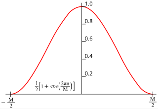
In signal processing and statistics, a window function is a mathematical function that is zero-valued outside of some chosen interval. Typically, windows functions are symmetric around the middle of the interval, approach a maximum in the middle, and taper away from the middle. Mathematically, when another function or waveform/data-sequence is "multiplied" by a window function, the product is also zero-valued outside the interval: all that is left is the part where they overlap, the "view through the window". Equivalently, and in actual practice, the segment of data within the window is first isolated, and then only that data is multiplied by the window function values. Thus, tapering, not segmentation, is the main purpose of window functions.
Forecasting is the process of making predictions based on past and present data. Later these can be compared (resolved) against what happens. For example, a company might estimate their revenue in the next year, then compare it against the actual results creating a variance actual analysis. Prediction is a similar but more general term. Forecasting might refer to specific formal statistical methods employing time series, cross-sectional or longitudinal data, or alternatively to less formal judgmental methods or the process of prediction and resolution itself. Usage can vary between areas of application: for example, in hydrology the terms "forecast" and "forecasting" are sometimes reserved for estimates of values at certain specific future times, while the term "prediction" is used for more general estimates, such as the number of times floods will occur over a long period.
In mathematics, the Hodge star operator or Hodge star is a linear map defined on the exterior algebra of a finite-dimensional oriented vector space endowed with a nondegenerate symmetric bilinear form. Applying the operator to an element of the algebra produces the Hodge dual of the element. This map was introduced by W. V. D. Hodge.
Multi-index notation is a mathematical notation that simplifies formulas used in multivariable calculus, partial differential equations and the theory of distributions, by generalising the concept of an integer index to an ordered tuple of indices.
In Bayesian probability theory, if, given a likelihood function , the posterior distribution is in the same probability distribution family as the prior probability distribution , the prior and posterior are then called conjugate distributions with respect to that likelihood function and the prior is called a conjugate prior for the likelihood function .
In probability theory, a distribution is said to be stable if a linear combination of two independent random variables with this distribution has the same distribution, up to location and scale parameters. A random variable is said to be stable if its distribution is stable. The stable distribution family is also sometimes referred to as the Lévy alpha-stable distribution, after Paul Lévy, the first mathematician to have studied it.
In probability theory, Hoeffding's inequality provides an upper bound on the probability that the sum of bounded independent random variables deviates from its expected value by more than a certain amount. Hoeffding's inequality was proven by Wassily Hoeffding in 1963.
In probability theory and statistics, the generalized extreme value (GEV) distribution is a family of continuous probability distributions developed within extreme value theory to combine the Gumbel, Fréchet and Weibull families also known as type I, II and III extreme value distributions. By the extreme value theorem the GEV distribution is the only possible limit distribution of properly normalized maxima of a sequence of independent and identically distributed random variables. Note that a limit distribution needs to exist, which requires regularity conditions on the tail of the distribution. Despite this, the GEV distribution is often used as an approximation to model the maxima of long (finite) sequences of random variables.
In statistics and econometrics, and in particular in time series analysis, an autoregressive integrated moving average (ARIMA) model is a generalization of an autoregressive moving average (ARMA) model. To better comprehend the data or to forecast upcoming series points, both of these models are fitted to time series data. ARIMA models are applied in some cases where data show evidence of non-stationarity in the sense of mean, where an initial differencing step can be applied one or more times to eliminate the non-stationarity of the mean function. When the seasonality shows in a time series, the seasonal-differencing could be applied to eliminate the seasonal component. Since the ARMA model, according to the Wold's decomposition theorem, is theoretically sufficient to describe a regular wide-sense stationary time series, we are motivated to make stationary a non-stationary time series, e.g., by using differencing, before we can use the ARMA model. Note that if the time series contains a predictable sub-process, the predictable component is treated as a non-zero-mean but periodic component in the ARIMA framework so that it is eliminated by the seasonal differencing.
In mathematics, the logarithmic mean is a function of two non-negative numbers which is equal to their difference divided by the logarithm of their quotient. This calculation is applicable in engineering problems involving heat and mass transfer.
In number theory, an average order of an arithmetic function is some simpler or better-understood function which takes the same values "on average".
The generalized normal distribution or generalized Gaussian distribution (GGD) is either of two families of parametric continuous probability distributions on the real line. Both families add a shape parameter to the normal distribution. To distinguish the two families, they are referred to below as "symmetric" and "asymmetric"; however, this is not a standard nomenclature.
In probability theory and statistics, the Poisson distribution is a discrete probability distribution that expresses the probability of a given number of events occurring in a fixed interval of time if these events occur with a known constant mean rate and independently of the time since the last event. It can also be used for the number of events in other types of intervals than time, and in dimension greater than 1.
In mathematics, a smooth maximum of an indexed family x1, ..., xn of numbers is a smooth approximation to the maximum function meaning a parametric family of functions such that for every α, the function is smooth, and the family converges to the maximum function as . The concept of smooth minimum is similarly defined. In many cases, a single family approximates both: maximum as the parameter goes to positive infinity, minimum as the parameter goes to negative infinity; in symbols, as and as . The term can also be used loosely for a specific smooth function that behaves similarly to a maximum, without necessarily being part of a parametrized family.
Generalized pencil-of-function method (GPOF), also known as matrix pencil method, is a signal processing technique for estimating a signal or extracting information with complex exponentials. Being similar to Prony and original pencil-of-function methods, it is generally preferred to those for its robustness and computational efficiency.
This page is based on this Wikipedia article Text is available under the CC BY-SA 4.0 license; additional terms may apply. Images, videos and audio are available under their respective licenses.