In probability theory and statistics, the binomial distribution with parameters n and p is the discrete probability distribution of the number of successes in a sequence of n independent experiments, each asking a yes–no question, and each with its own Boolean-valued outcome: success or failure. A single success/failure experiment is also called a Bernoulli trial or Bernoulli experiment, and a sequence of outcomes is called a Bernoulli process; for a single trial, i.e., n = 1, the binomial distribution is a Bernoulli distribution. The binomial distribution is the basis for the popular binomial test of statistical significance.

In probability theory and statistics, the cumulative distribution function (CDF) of a real-valued random variable , or just distribution function of , evaluated at , is the probability that will take a value less than or equal to .

In statistics, the Kolmogorov–Smirnov test is a nonparametric test of the equality of continuous, one-dimensional probability distributions that can be used to test whether a sample came from a given reference probability distribution, or to test whether two samples came from the same distribution. Intuitively, the test provides a method to qualitatively answer the question "How likely is it that we would see a collection of samples like this if they were drawn from that probability distribution?" or, in the second case, "How likely is it that we would see two sets of samples like this if they were drawn from the same probability distribution?". It is named after Andrey Kolmogorov and Nikolai Smirnov.
In probability theory, the central limit theorem (CLT) states that, under appropriate conditions, the distribution of a normalized version of the sample mean converges to a standard normal distribution. This holds even if the original variables themselves are not normally distributed. There are several versions of the CLT, each applying in the context of different conditions.

The Pareto distribution, named after the Italian civil engineer, economist, and sociologist Vilfredo Pareto, is a power-law probability distribution that is used in description of social, quality control, scientific, geophysical, actuarial, and many other types of observable phenomena; the principle originally applied to describing the distribution of wealth in a society, fitting the trend that a large portion of wealth is held by a small fraction of the population. The Pareto principle or "80-20 rule" stating that 80% of outcomes are due to 20% of causes was named in honour of Pareto, but the concepts are distinct, and only Pareto distributions with shape value of log45 ≈ 1.16 precisely reflect it. Empirical observation has shown that this 80-20 distribution fits a wide range of cases, including natural phenomena and human activities.

In probability theory, a log-normal (or lognormal) distribution is a continuous probability distribution of a random variable whose logarithm is normally distributed. Thus, if the random variable X is log-normally distributed, then Y = ln(X) has a normal distribution. Equivalently, if Y has a normal distribution, then the exponential function of Y, X = exp(Y), has a log-normal distribution. A random variable which is log-normally distributed takes only positive real values. It is a convenient and useful model for measurements in exact and engineering sciences, as well as medicine, economics and other topics (e.g., energies, concentrations, lengths, prices of financial instruments, and other metrics).

In probability theory, the law of large numbers (LLN) is a mathematical theorem that states that the average of the results obtained from a large number of independent and identical random samples converges to the true value, if it exists. More formally, the LLN states that given a sample of independent and identically distributed values, the sample mean converges to the true mean.

In probability theory and statistics, the Rayleigh distribution is a continuous probability distribution for nonnegative-valued random variables. Up to rescaling, it coincides with the chi distribution with two degrees of freedom. The distribution is named after Lord Rayleigh.

In probability theory and statistics, the Gumbel distribution is used to model the distribution of the maximum of a number of samples of various distributions.

In probability theory, a distribution is said to be stable if a linear combination of two independent random variables with this distribution has the same distribution, up to location and scale parameters. A random variable is said to be stable if its distribution is stable. The stable distribution family is also sometimes referred to as the Lévy alpha-stable distribution, after Paul Lévy, the first mathematician to have studied it.

In statistics, a consistent estimator or asymptotically consistent estimator is an estimator—a rule for computing estimates of a parameter θ0—having the property that as the number of data points used increases indefinitely, the resulting sequence of estimates converges in probability to θ0. This means that the distributions of the estimates become more and more concentrated near the true value of the parameter being estimated, so that the probability of the estimator being arbitrarily close to θ0 converges to one.

In probability theory and statistics, the continuous uniform distributions or rectangular distributions are a family of symmetric probability distributions. Such a distribution describes an experiment where there is an arbitrary outcome that lies between certain bounds. The bounds are defined by the parameters, and which are the minimum and maximum values. The interval can either be closed or open. Therefore, the distribution is often abbreviated where stands for uniform distribution. The difference between the bounds defines the interval length; all intervals of the same length on the distribution's support are equally probable. It is the maximum entropy probability distribution for a random variable under no constraint other than that it is contained in the distribution's support.
In mathematics and statistics, an asymptotic distribution is a probability distribution that is in a sense the "limiting" distribution of a sequence of distributions. One of the main uses of the idea of an asymptotic distribution is in providing approximations to the cumulative distribution functions of statistical estimators.
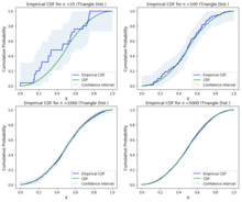
In the theory of probability, the Glivenko–Cantelli theorem, named after Valery Ivanovich Glivenko and Francesco Paolo Cantelli, describes the asymptotic behaviour of the empirical distribution function as the number of independent and identically distributed observations grows. Specifically, the empirical distribution function converges uniformly to the true distribution function almost surely.
In probability theory, heavy-tailed distributions are probability distributions whose tails are not exponentially bounded: that is, they have heavier tails than the exponential distribution. In many applications it is the right tail of the distribution that is of interest, but a distribution may have a heavy left tail, or both tails may be heavy.

In the theory of probability and statistics, the Dvoretzky–Kiefer–Wolfowitz–Massart inequality provides a bound on the worst case distance of an empirically determined distribution function from its associated population distribution function. It is named after Aryeh Dvoretzky, Jack Kiefer, and Jacob Wolfowitz, who in 1956 proved the inequality
In probability theory, the probability integral transform relates to the result that data values that are modeled as being random variables from any given continuous distribution can be converted to random variables having a standard uniform distribution. This holds exactly provided that the distribution being used is the true distribution of the random variables; if the distribution is one fitted to the data, the result will hold approximately in large samples.

In probability and statistics, the quantile function outputs the value of a random variable such that its probability is less than or equal to an input probability value. Intuitively, the quantile function associates with a range at and below a probability input the likelihood that a random variable is realized in that range for some probability distribution. It is also called the percentile function, percent-point function, inverse cumulative distribution function or inverse distribution function.
In statistics, the Fisher–Tippett–Gnedenko theorem is a general result in extreme value theory regarding asymptotic distribution of extreme order statistics. The maximum of a sample of iid random variables after proper renormalization can only converge in distribution to one of only 3 possible distribution families: the Gumbel distribution, the Fréchet distribution, or the Weibull distribution. Credit for the extreme value theorem and its convergence details are given to Fréchet (1927), Fisher and Tippett (1928), Mises (1936), and Gnedenko (1943).
In probability theory, the Komlós–Major–Tusnády approximation refers to one of the two strong embedding theorems: 1) approximation of random walk by a standard Brownian motion constructed on the same probability space, and 2) an approximation of the empirical process by a Brownian bridge constructed on the same probability space. It is named after Hungarian mathematicians János Komlós, Gábor Tusnády, and Péter Major, who proved it in 1975.