Mean

Last updated April 20, 2024

A mean is a numeric quantity representing the center of a collection of numbers and is intermediate to the extreme values of a set of numbers.^[1] There are several kinds of means (or "measures of central tendency") in mathematics, especially in statistics. Each attempts to summarize or typify a given group of data, illustrating the magnitude and sign of the data set. Which of these measures is most illuminating depends on what is being measured, and on context and purpose.

The arithmetic mean , also known as "arithmetic average", is the sum of the values divided by the number of values. The arithmetic mean of a set of numbers x₁, x₂, ..., x_n is typically denoted using an overhead bar, ${\bar {x}}$ .^{[note 1]} If the numbers are from observing a sample of a larger group, the arithmetic mean is termed the sample mean ( ${\bar {x}}$ ) to distinguish it from the group mean (or expected value) of the underlying distribution, denoted $\mu$ or $\mu _{x}$ .^{[note 2]}^[2]

Outside probability and statistics, a wide range of other notions of mean are often used in geometry and mathematical analysis; examples are given below.

Types of means

Pythagorean means

Arithmetic mean (AM)

The arithmetic mean (or simply mean or average) of a list of numbers, is the sum of all of the numbers divided by the number of numbers. Similarly, the mean of a sample $x_{1},x_{2},\ldots ,x_{n}$ , usually denoted by ${\bar {x}}$ , is the sum of the sampled values divided by the number of items in the sample.

{\bar {x}}={\frac {1}{n}}\left(\sum _{i=1}^{n}{x_{i}}\right)={\frac {x_{1}+x_{2}+\cdots +x_{n}}{n}}

For example, the arithmetic mean of five values: 4, 36, 45, 50, 75 is:

{\frac {4+36+45+50+75}{5}}={\frac {210}{5}}=42.

Geometric mean (GM)

The geometric mean is an average that is useful for sets of positive numbers, that are interpreted according to their product (as is the case with rates of growth) and not their sum (as is the case with the arithmetic mean):

{\bar {x}}=\left(\prod _{i=1}^{n}{x_{i}}\right)^{\frac {1}{n}}=\left(x_{1}x_{2}\cdots x_{n}\right)^{\frac {1}{n}}

^[1]

For example, the geometric mean of five values: 4, 36, 45, 50, 75 is:

(4\times 36\times 45\times 50\times 75)^{\frac {1}{5}}={\sqrt[{5}]{24\;300\;000}}=30.

Harmonic mean (HM)

The harmonic mean is an average which is useful for sets of numbers which are defined in relation to some unit, as in the case of speed (i.e., distance per unit of time):

{\bar {x}}=n\left(\sum _{i=1}^{n}{\frac {1}{x_{i}}}\right)^{-1}

For example, the harmonic mean of the five values: 4, 36, 45, 50, 75 is

{\frac {5}{{\tfrac {1}{4}}+{\tfrac {1}{36}}+{\tfrac {1}{45}}+{\tfrac {1}{50}}+{\tfrac {1}{75}}}}={\frac {5}{\;{\tfrac {1}{3}}\;}}=15.

If we have five pumps that can empty a tank of a certain size in respectively 4, 36, 45, 50, and 75 minutes, then the harmonic mean of $15$ tells us that these five different pumps working together will pump at the same rate as much as five pumps that can each empty the tank in $15$ minutes.

Relationship between AM, GM, and HM

AM, GM, and HM satisfy these inequalities:

\mathrm {AM} \geq \mathrm {GM} \geq \mathrm {HM} \,

Equality holds if all the elements of the given sample are equal.

Statistical location

In descriptive statistics, the mean may be confused with the median, mode or mid-range, as any of these may incorrectly be called an "average" (more formally, a measure of central tendency). The mean of a set of observations is the arithmetic average of the values; however, for skewed distributions, the mean is not necessarily the same as the middle value (median), or the most likely value (mode). For example, mean income is typically skewed upwards by a small number of people with very large incomes, so that the majority have an income lower than the mean. By contrast, the median income is the level at which half the population is below and half is above. The mode income is the most likely income and favors the larger number of people with lower incomes. While the median and mode are often more intuitive measures for such skewed data, many skewed distributions are in fact best described by their mean, including the exponential and Poisson distributions.

Mean of a probability distribution

The mean of a probability distribution is the long-run arithmetic average value of a random variable having that distribution. If the random variable is denoted by $X$ , then the mean is also known as the expected value of $X$ (denoted $E(X)$ ). For a discrete probability distribution, the mean is given by $\textstyle \sum xP(x)$ , where the sum is taken over all possible values of the random variable and $P(x)$ is the probability mass function. For a continuous distribution, the mean is $\textstyle \int _{-\infty }^{\infty }xf(x)\,dx$ , where $f(x)$ is the probability density function.^[4] In all cases, including those in which the distribution is neither discrete nor continuous, the mean is the Lebesgue integral of the random variable with respect to its probability measure. The mean need not exist or be finite; for some probability distributions the mean is infinite ( $+ \infty$ or $- \infty$ ), while for others the mean is undefined.

Generalized means

Power mean

The generalized mean, also known as the power mean or Hölder mean, is an abstraction of the quadratic, arithmetic, geometric, and harmonic means. It is defined for a set of n positive numbers x_i by

${\bar {x}}(m)=\left({\frac {1}{n}}\sum _{i=1}^{n}x_{i}^{m}\right)^{\frac {1}{m}}$ ^[1]

By choosing different values for the parameter m, the following types of means are obtained:

$\lim _{m\to \infty }$: maximum of $x_{i}$
$\lim _{m\to 2}$: quadratic mean
$\lim _{m\to 1}$: arithmetic mean
$\lim _{m\to 0}$: geometric mean
$\lim _{m\to -1}$: harmonic mean
$\lim _{m\to -\infty }$: minimum of $x_{i}$

f-mean

This can be generalized further as the generalized $f$ -mean

{\bar {x}}=f^{-1}\left({{\frac {1}{n}}\sum _{i=1}^{n}{f\left(x_{i}\right)}}\right)

and again a suitable choice of an invertible $f$ will give

$f(x)=x^{m}$	power mean,
$f(x)=x$	arithmetic mean,
$f(x)=\ln(x)$	geometric mean.
$f(x)=x^{-1}={\frac {1}{x}}$	harmonic mean,

Weighted arithmetic mean

The weighted arithmetic mean (or weighted average) is used if one wants to combine average values from different sized samples of the same population:

{\bar {x}}={\frac {\sum _{i=1}^{n}{w_{i}{\bar {x_{i}}}}}{\sum _{i=1}^{n}w_{i}}}.

^[1]

Where ${\bar {x_{i}}}$ and $w_{i}$ are the mean and size of sample $i$ respectively. In other applications, they represent a measure for the reliability of the influence upon the mean by the respective values.

Truncated mean

Sometimes, a set of numbers might contain outliers (i.e., data values which are much lower or much higher than the others). Often, outliers are erroneous data caused by artifacts. In this case, one can use a truncated mean. It involves discarding given parts of the data at the top or the bottom end, typically an equal amount at each end and then taking the arithmetic mean of the remaining data. The number of values removed is indicated as a percentage of the total number of values.

Interquartile mean

The interquartile mean is a specific example of a truncated mean. It is simply the arithmetic mean after removing the lowest and the highest quarter of values.

{\bar {x}}={\frac {2}{n}}\;\sum _{i={\frac {n}{4}}+1}^{{\frac {3}{4}}n}\!\!x_{i}

assuming the values have been ordered, so is simply a specific example of a weighted mean for a specific set of weights.

Mean of a function

In some circumstances, mathematicians may calculate a mean of an infinite (or even an uncountable) set of values. This can happen when calculating the mean value $y_{\text{avg}}$ of a function $f(x)$ . Intuitively, a mean of a function can be thought of as calculating the area under a section of a curve, and then dividing by the length of that section. This can be done crudely by counting squares on graph paper, or more precisely by integration. The integration formula is written as:

y_{\text{avg}}(a,b)={\frac {1}{b-a}}\int \limits _{a}^{b}\!f(x)\,dx

In this case, care must be taken to make sure that the integral converges. But the mean may be finite even if the function itself tends to infinity at some points.

Mean of angles and cyclical quantities

Angles, times of day, and other cyclical quantities require modular arithmetic to add and otherwise combine numbers. In all these situations, there will not be a unique mean. For example, the times an hour before and after midnight are equidistant to both midnight and noon. It is also possible that no mean exists. Consider a color wheel—there is no mean to the set of all colors. In these situations, you must decide which mean is most useful. You can do this by adjusting the values before averaging, or by using a specialized approach for the mean of circular quantities.

Fréchet mean

The Fréchet mean gives a manner for determining the "center" of a mass distribution on a surface or, more generally, Riemannian manifold. Unlike many other means, the Fréchet mean is defined on a space whose elements cannot necessarily be added together or multiplied by scalars. It is sometimes also known as the Karcher mean (named after Hermann Karcher).

Triangular sets

In geometry, there are thousands of different definitions for the center of a triangle that can all be interpreted as the mean of a triangular set of points in the plane.^{[ citation needed ]}

Swanson's rule

This is an approximation to the mean for a moderately skewed distribution.^[5] It is used in hydrocarbon exploration and is defined as:

m=0.3P_{10}+0.4P_{50}+0.3P_{90}

where ${\textstyle P_{10}}$ , ${\textstyle P_{50}}$ and ${\textstyle P_{90}}$ are the 10th, 50th and 90th percentiles of the distribution, respctively.

Notes

↑ Pronounced "x bar".
↑ Greek letter μ, for "mean", pronounced /'mjuː/.

Related Research Articles

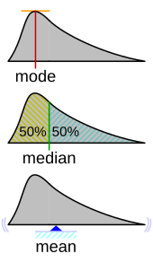
In mathematics and statistics, the arithmetic mean, arithmetic average, or just the mean or average is the sum of a collection of numbers divided by the count of numbers in the collection. The collection is often a set of results from an experiment, an observational study, or a survey. The term "arithmetic mean" is preferred in some mathematics and statistics contexts because it helps distinguish it from other types of means, such as geometric and harmonic.

The Cauchy distribution, named after Augustin Cauchy, is a continuous probability distribution. It is also known, especially among physicists, as the Lorentz distribution, Cauchy–Lorentz distribution, Lorentz(ian) function, or Breit–Wigner distribution. The Cauchy distribution $is the distribution of the x -intercept of a ray issuing from with a uniformly distributed angle. It is also the distribution of the ratio of two independent normally distributed random variables with mean zero.$

In probability theory, the expected value is a generalization of the weighted average. Informally, the expected value is the arithmetic mean of the possible values a random variable can take, weighted by the probability of those outcomes. Since it is obtained through arithmetic, the expected value sometimes may not even be included in the sample data set; it is not the value you would "expect" to get in reality.

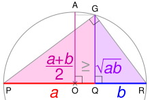
In mathematics, the geometric mean is a mean or average which indicates a central tendency of a finite set of real numbers by using the product of their values. The geometric mean is defined as the $n$ th root of the product of $n$ numbers, i.e., for a set of numbers $a 1, a 2, ..., a n$ , the geometric mean is defined as

In mathematics, generalized means are a family of functions for aggregating sets of numbers. These include as special cases the Pythagorean means.

In mathematics, the harmonic mean is one of several kinds of average, and in particular, one of the Pythagorean means. It is sometimes appropriate for situations when the average rate is desired.

In statistics, a normal distribution or Gaussian distribution is a type of continuous probability distribution for a real-valued random variable. The general form of its probability density function is

In statistics, the standard deviation is a measure of the amount of variation of a random variable expected about its mean. A low standard deviation indicates that the values tend to be close to the mean of the set, while a high standard deviation indicates that the values are spread out over a wider range. The standard deviation is commonly used in the determination of what constitutes an outlier and what does not.

In probability theory and statistics, variance is the expected value of the squared deviation from the mean of a random variable. The standard deviation (SD) is obtained as the square root of the variance. Variance is a measure of dispersion, meaning it is a measure of how far a set of numbers is spread out from their average value. It is the second central moment of a distribution, and the covariance of the random variable with itself, and it is often represented by $,,,, or .$

In probability theory, the central limit theorem (CLT) states that, under appropriate conditions, the distribution of a normalized version of the sample mean converges to a standard normal distribution. This holds even if the original variables themselves are not normally distributed. There are several versions of the CLT, each applying in the context of different conditions.

<span class="mw-page-title-main">Log-normal distribution</span> Probability distribution

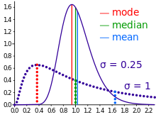
In probability theory, a log-normal (or lognormal) distribution is a continuous probability distribution of a random variable whose logarithm is normally distributed. Thus, if the random variable $X$ is log-normally distributed, then $Y = ln(X)$ has a normal distribution. Equivalently, if $Y$ has a normal distribution, then the exponential function of $Y$ , $X = exp(Y)$ , has a log-normal distribution. A random variable which is log-normally distributed takes only positive real values. It is a convenient and useful model for measurements in exact and engineering sciences, as well as medicine, economics and other topics (e.g., energies, concentrations, lengths, prices of financial instruments, and other metrics).

In probability theory and statistics, the chi-squared distribution with $degrees of freedom is the distribution of a sum of the squares of independent standard normal random variables. The chi-squared distribution is a special case of the gamma distribution and is one of the most widely used probability distributions in inferential statistics, notably in hypothesis testing and in construction of confidence intervals. This distribution is sometimes called the central chi-squared distribution, a special case of the more general noncentral chi-squared distribution.$

In probability theory, the law of large numbers (LLN) is a mathematical theorem that states that the average of the results obtained from a large number of independent and identical random samples converges to the true value, if it exists. More formally, the LLN states that given a sample of independent and identically distributed values, the sample mean converges to the true mean.

In probability theory and statistics, the beta distribution is a family of continuous probability distributions defined on the interval [0, 1] or in terms of two positive parameters, denoted by alpha (α) and beta (β), that appear as exponents of the variable and its complement to 1, respectively, and control the shape of the distribution.

<span class="mw-page-title-main">Harmonic number</span> Sum of the first n whole number reciprocals; 1/1 + 1/2 + 1/3 + ... + 1/n

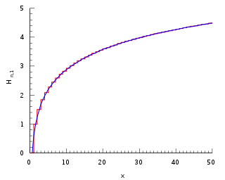
In mathematics, the $n$ -th harmonic number is the sum of the reciprocals of the first $n$ natural numbers:

In statistics, the Pearson correlation coefficient (PCC) is a correlation coefficient that measures linear correlation between two sets of data. It is the ratio between the covariance of two variables and the product of their standard deviations; thus, it is essentially a normalized measurement of the covariance, such that the result always has a value between −1 and 1. As with covariance itself, the measure can only reflect a linear correlation of variables, and ignores many other types of relationships or correlations. As a simple example, one would expect the age and height of a sample of teenagers from a high school to have a Pearson correlation coefficient significantly greater than 0, but less than 1.

In probability theory and statistics, the continuous uniform distributions or rectangular distributions are a family of symmetric probability distributions. Such a distribution describes an experiment where there is an arbitrary outcome that lies between certain bounds. The bounds are defined by the parameters, $and which are the minimum and maximum values. The interval can either be closed or open. Therefore, the distribution is often abbreviated where stands for uniform distribution. The difference between the bounds defines the interval length; all intervals of the same length on the distribution's support are equally probable. It is the maximum entropy probability distribution for a random variable under no constraint other than that it is contained in the distribution's support.$

In mathematics, a contraharmonic mean is a function complementary to the harmonic mean. The contraharmonic mean is a special case of the Lehmer mean, $, where p = 2.$

The sample mean or empirical mean, and the sample covariance or empirical covariance are statistics computed from a sample of data on one or more random variables.

A geometric progression, also known as a geometric sequence, is a mathematical sequence of non-zero numbers where each term after the first is found by multiplying the previous one by a fixed, non-zero number called the common ratio. For example, the sequence 2, 6, 18, 54, ... is a geometric progression with common ratio 3. Similarly 10, 5, 2.5, 1.25, ... is a geometric sequence with common ratio 1/2.

References

1 2 3 4 "Mean | mathematics". Encyclopedia Britannica. Retrieved 2020-08-21.
↑ Underhill, L.G.; Bradfield d. (1998) Introstat, Juta and Company Ltd. ISBN 0-7021-3838-X p. 181
↑ "AP Statistics Review - Density Curves and the Normal Distributions". Archived from the original on 2 April 2015. Retrieved 16 March 2015.
↑ Weisstein, Eric W. "Population Mean". mathworld.wolfram.com. Retrieved 2020-08-21.
↑ Hurst A, Brown GC, Swanson RI (2000) Swanson's 30-40-30 Rule. American Association of Petroleum Geologists Bulletin 84(12) 1883-1891

This page is based on this Wikipedia article
Text is available under the CC BY-SA 4.0 license; additional terms may apply.
Images, videos and audio are available under their respective licenses.

[2] Pronounced "x bar".

[3] Greek letter μ, for "mean", pronounced /'mjuː/.

[:2-1] 1 2 3 4 "Mean | mathematics". Encyclopedia Britannica. Retrieved 2020-08-21.

[4] Underhill, L.G.; Bradfield d. (1998) Introstat, Juta and Company Ltd. ISBN 0-7021-3838-X p. 181

[5] "AP Statistics Review - Density Curves and the Normal Distributions". Archived from the original on 2 April 2015. Retrieved 16 March 2015.

[:1-6] Weisstein, Eric W. "Population Mean". mathworld.wolfram.com. Retrieved 2020-08-21.

[Hurst2000-7] Hurst A, Brown GC, Swanson RI (2000) Swanson's 30-40-30 Rule. American Association of Petroleum Geologists Bulletin 84(12) 1883-1891

[1]

[note 1]

[note 2]

[2]

[4]

[5]