A histogram is a visual representation of the distribution of quantitative data. The term was first introduced by Karl Pearson. To construct a histogram, the first step is to "bin" the range of values— divide the entire range of values into a series of intervals—and then count how many values fall into each interval. The bins are usually specified as consecutive, non-overlapping intervals of a variable. The bins (intervals) are adjacent and are typically of equal size.
The following outline is provided as an overview of and topical guide to statistics:
Nonparametric statistics is a type of statistical analysis that makes minimal assumptions about the underlying distribution of the data being studied. Often these models are infinite-dimensional, rather than finite dimensional, as is parametric statistics. Nonparametric statistics can be used for descriptive statistics or statistical inference. Nonparametric tests are often used when the assumptions of parametric tests are evidently violated.

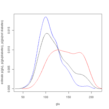
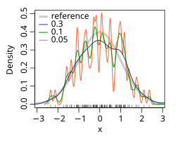
In statistics, kernel density estimation (KDE) is the application of kernel smoothing for probability density estimation, i.e., a non-parametric method to estimate the probability density function of a random variable based on kernels as weights. KDE answers a fundamental data smoothing problem where inferences about the population are made, based on a finite data sample. In some fields such as signal processing and econometrics it is also termed the Parzen–Rosenblatt window method, after Emanuel Parzen and Murray Rosenblatt, who are usually credited with independently creating it in its current form. One of the famous applications of kernel density estimation is in estimating the class-conditional marginal densities of data when using a naive Bayes classifier, which can improve its prediction accuracy.
This glossary of statistics and probability is a list of definitions of terms and concepts used in the mathematical sciences of statistics and probability, their sub-disciplines, and related fields. For additional related terms, see Glossary of mathematics and Glossary of experimental design.
In statistics, semiparametric regression includes regression models that combine parametric and nonparametric models. They are often used in situations where the fully nonparametric model may not perform well or when the researcher wants to use a parametric model but the functional form with respect to a subset of the regressors or the density of the errors is not known. Semiparametric regression models are a particular type of semiparametric modelling and, since semiparametric models contain a parametric component, they rely on parametric assumptions and may be misspecified and inconsistent, just like a fully parametric model.
Bootstrapping is any test or metric that uses random sampling with replacement, and falls under the broader class of resampling methods. Bootstrapping assigns measures of accuracy to sample estimates. This technique allows estimation of the sampling distribution of almost any statistic using random sampling methods.
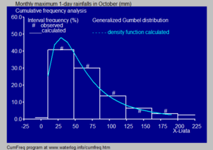
In probability theory, heavy-tailed distributions are probability distributions whose tails are not exponentially bounded: that is, they have heavier tails than the exponential distribution. In many applications it is the right tail of the distribution that is of interest, but a distribution may have a heavy left tail, or both tails may be heavy.
The term kernel is used in statistical analysis to refer to a window function. The term "kernel" has several distinct meanings in different branches of statistics.
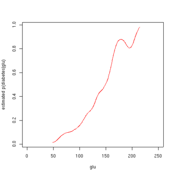
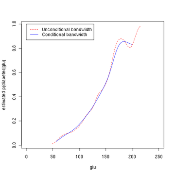
In statistics, kernel regression is a non-parametric technique to estimate the conditional expectation of a random variable. The objective is to find a non-linear relation between a pair of random variables X and Y.
A utilization distribution is a probability distribution giving the probability density that an animal is found at a given point in space. It is estimated from data sampling the location of an individual or individuals in space over a period of time using, for example, telemetry or GPS based methods.
Mean shift is a non-parametric feature-space mathematical analysis technique for locating the maxima of a density function, a so-called mode-seeking algorithm. Application domains include cluster analysis in computer vision and image processing.
A kernel smoother is a statistical technique to estimate a real valued function as the weighted average of neighboring observed data. The weight is defined by the kernel, such that closer points are given higher weights. The estimated function is smooth, and the level of smoothness is set by a single parameter. Kernel smoothing is a type of weighted moving average.
In various science/engineering applications, such as independent component analysis, image analysis, genetic analysis, speech recognition, manifold learning, and time delay estimation it is useful to estimate the differential entropy of a system or process, given some observations.
Kernel density estimation is a nonparametric technique for density estimation i.e., estimation of probability density functions, which is one of the fundamental questions in statistics. It can be viewed as a generalisation of histogram density estimation with improved statistical properties. Apart from histograms, other types of density estimators include parametric, spline, wavelet and Fourier series. Kernel density estimators were first introduced in the scientific literature for univariate data in the 1950s and 1960s and subsequently have been widely adopted. It was soon recognised that analogous estimators for multivariate data would be an important addition to multivariate statistics. Based on research carried out in the 1990s and 2000s, multivariate kernel density estimation has reached a level of maturity comparable to its univariate counterparts.
In machine learning, the kernel embedding of distributions comprises a class of nonparametric methods in which a probability distribution is represented as an element of a reproducing kernel Hilbert space (RKHS). A generalization of the individual data-point feature mapping done in classical kernel methods, the embedding of distributions into infinite-dimensional feature spaces can preserve all of the statistical features of arbitrary distributions, while allowing one to compare and manipulate distributions using Hilbert space operations such as inner products, distances, projections, linear transformations, and spectral analysis. This learning framework is very general and can be applied to distributions over any space on which a sensible kernel function may be defined. For example, various kernels have been proposed for learning from data which are: vectors in , discrete classes/categories, strings, graphs/networks, images, time series, manifolds, dynamical systems, and other structured objects. The theory behind kernel embeddings of distributions has been primarily developed by Alex Smola, Le Song , Arthur Gretton, and Bernhard Schölkopf. A review of recent works on kernel embedding of distributions can be found in.
In machine learning, a probabilistic classifier is a classifier that is able to predict, given an observation of an input, a probability distribution over a set of classes, rather than only outputting the most likely class that the observation should belong to. Probabilistic classifiers provide classification that can be useful in its own right or when combining classifiers into ensembles.
Let be independent, identically distributed real-valued random variables with common characteristic function . The empirical characteristic function (ECF) defined as
Èlizbar Nadaraya is a Georgian mathematician who is currently a Full Professor and the Chair of the Theory of Probability and Mathematical Statistics at the Tbilisi State University. He developed the Nadaraya-Watson estimator along with Geoffrey Watson, which proposes estimating the conditional expectation of a random variable as a locally weighted average using a kernel as a weighting function.