Probability distribution fitting

Last updated

Probability distribution fitting or simply distribution fitting is the fitting of a probability distribution to a series of data concerning the repeated measurement of a variable phenomenon. The aim of distribution fitting is to predict the probability or to forecast the frequency of occurrence of the magnitude of the phenomenon in a certain interval.

Contents

There are many probability distributions (see list of probability distributions) of which some can be fitted more closely to the observed frequency of the data than others, depending on the characteristics of the phenomenon and of the distribution. The distribution giving a close fit is supposed to lead to good predictions. In distribution fitting, therefore, one needs to select a distribution that suits the data well.

Selection of distribution

Different shapes of the symmetrical normal distribution depending on mean m and variance s Normal Distribution PDF.svg
Different shapes of the symmetrical normal distribution depending on mean μ and variance σ

The selection of the appropriate distribution depends on the presence or absence of symmetry of the data set with respect to the central tendency.

Symmetrical distributions

When the data are symmetrically distributed around the mean while the frequency of occurrence of data farther away from the mean diminishes, one may for example select the normal distribution, the logistic distribution, or the Student's t-distribution. The first two are very similar, while the last, with one degree of freedom, has "heavier tails" meaning that the values farther away from the mean occur relatively more often (i.e. the kurtosis is higher). The Cauchy distribution is also symmetric.

Skew distributions to the right

Skewness to left and right Negative and positive skew diagrams (English).svg
Skewness to left and right

When the larger values tend to be farther away from the mean than the smaller values, one has a skew distribution to the right (i.e. there is positive skewness), one may for example select the log-normal distribution (i.e. the log values of the data are normally distributed), the log-logistic distribution (i.e. the log values of the data follow a logistic distribution), the Gumbel distribution, the exponential distribution, the Pareto distribution, the Weibull distribution, the Burr distribution, or the Fréchet distribution. The last four distributions are bounded to the left.

Skew distributions to the left

When the smaller values tend to be farther away from the mean than the larger values, one has a skew distribution to the left (i.e. there is negative skewness), one may for example select the square-normal distribution (i.e. the normal distribution applied to the square of the data values), [1] the inverted (mirrored) Gumbel distribution, [1] the Dagum distribution (mirrored Burr distribution), or the Gompertz distribution, which is bounded to the left.

Techniques of fitting

The following techniques of distribution fitting exist: [2]

For example, the parameter (the expectation) can be estimated by the mean of the data and the parameter (the variance) can be estimated from the standard deviation of the data. The mean is found as , where is the data value and the number of data, while the standard deviation is calculated as . With these parameters many distributions, e.g. the normal distribution, are completely defined.
Cumulative Gumbel distribution fitted to maximum one-day October rainfalls in Suriname by the regression method with added confidence band using cumfreq FitGumbelDistr.tif
Cumulative Gumbel distribution fitted to maximum one-day October rainfalls in Suriname by the regression method with added confidence band using cumfreq
For example, the cumulative Gumbel distribution can be linearized to , where is the data variable and , with being the cumulative probability, i.e. the probability that the data value is less than . Thus, using the plotting position for , one finds the parameters and from a linear regression of on , and the Gumbel distribution is fully defined.

Generalization of distributions

It is customary to transform data logarithmically to fit symmetrical distributions (like the normal and logistic) to data obeying a distribution that is positively skewed (i.e. skew to the right, with mean > mode, and with a right hand tail that is longer than the left hand tail), see lognormal distribution and the loglogistic distribution. A similar effect can be achieved by taking the square root of the data.

To fit a symmetrical distribution to data obeying a negatively skewed distribution (i.e. skewed to the left, with mean < mode, and with a right hand tail this is shorter than the left hand tail) one could use the squared values of the data to accomplish the fit.

More generally one can raise the data to a power p in order to fit symmetrical distributions to data obeying a distribution of any skewness, whereby p < 1 when the skewness is positive and p > 1 when the skewness is negative. The optimal value of p is to be found by a numerical method. The numerical method may consist of assuming a range of p values, then applying the distribution fitting procedure repeatedly for all the assumed p values, and finally selecting the value of p for which the sum of squares of deviations of calculated probabilities from measured frequencies (chi squared) is minimum, as is done in CumFreq.

The generalization enhances the flexibility of probability distributions and increases their applicability in distribution fitting. [6]

The versatility of generalization makes it possible, for example, to fit approximately normally distributed data sets to a large number of different probability distributions, [7] while negatively skewed distributions can be fitted to square normal and mirrored Gumbel distributions. [8]

Inversion of skewness

(A) Gumbel probability distribution skew to right and (B) Gumbel mirrored skew to left Gumbel distribution and Gumbel mirrored.png
(A) Gumbel probability distribution skew to right and (B) Gumbel mirrored skew to left

Skewed distributions can be inverted (or mirrored) by replacing in the mathematical expression of the cumulative distribution function (F) by its complement: F'=1-F, obtaining the complementary distribution function (also called survival function) that gives a mirror image. In this manner, a distribution that is skewed to the right is transformed into a distribution that is skewed to the left and vice versa.

Example. The F-expression of the positively skewed Gumbel distribution is: F=exp[-exp{-(X-u)/0.78s}], where u is the mode (i.e. the value occurring most frequently) and s is the standard deviation. The Gumbel distribution can be transformed using F'=1-exp[-exp{-(x-u)/0.78s}] . This transformation yields the inverse, mirrored, or complementary Gumbel distribution that may fit a data series obeying a negatively skewed distribution.

The technique of skewness inversion increases the number of probability distributions available for distribution fitting and enlarges the distribution fitting opportunities.

Shifting of distributions

Some probability distributions, like the exponential, do not support negative data values (X). Yet, when negative data are present, such distributions can still be used replacing X by Y=X-Xm, where Xm is the minimum value of X. This replacement represents a shift of the probability distribution in positive direction, i.e. to the right, because Xm is negative. After completing the distribution fitting of Y, the corresponding X-values are found from X=Y+Xm, which represents a back-shift of the distribution in negative direction, i.e. to the left.
The technique of distribution shifting augments the chance to find a properly fitting probability distribution.

Composite distributions

Composite (discontinuous) distribution with confidence belt SanLor.jpg
Composite (discontinuous) distribution with confidence belt

The option exists to use two different probability distributions, one for the lower data range, and one for the higher like for example the Laplace distribution. The ranges are separated by a break-point. The use of such composite (discontinuous) probability distributions can be opportune when the data of the phenomenon studied were obtained under two sets different conditions. [6]

Uncertainty of prediction

Uncertainty analysis with confidence belts using the binomial distribution BinomialConfBelts.jpg
Uncertainty analysis with confidence belts using the binomial distribution

Predictions of occurrence based on fitted probability distributions are subject to uncertainty, which arises from the following conditions:

Variations of nine return period curves of 50-year samples from a theoretical 1000 year record (base line), data from Benson SampleFreqCurves.tif
Variations of nine return period curves of 50-year samples from a theoretical 1000 year record (base line), data from Benson

An estimate of the uncertainty in the first and second case can be obtained with the binomial probability distribution using for example the probability of exceedance Pe (i.e. the chance that the event X is larger than a reference value Xr of X) and the probability of non-exceedance Pn (i.e. the chance that the event X is smaller than or equal to the reference value Xr, this is also called cumulative probability). In this case there are only two possibilities: either there is exceedance or there is non-exceedance. This duality is the reason that the binomial distribution is applicable.

With the binomial distribution one can obtain a prediction interval. Such an interval also estimates the risk of failure, i.e. the chance that the predicted event still remains outside the confidence interval. The confidence or risk analysis may include the return period T=1/Pe as is done in hydrology.

Variance of Bayesian fitted probability functions

A Bayesian approach can be used for fitting a model having a prior distribution for the parameter . When one has samples that are independently drawn from the underlying distribution then one can derive the so-called posterior distribution . This posterior can be used to update the probability mass function for a new sample given the observations , one obtains

.

The variance of the newly obtained probability mass function can also be determined. The variance for a Bayesian probability mass function can be defined as

.

This expression for the variance can be substantially simplified (assuming independently drawn samples). Defining the "self probability mass function" as

,

one obtains for the variance [12]

.

The expression for variance involves an additional fit that includes the sample of interest.

List of probability distributions ranked by goodness of fit CumList.png
List of probability distributions ranked by goodness of fit
Histogram and probability density of a data set fitting the GEV distribution GEVdistrHistogr+Density.png
Histogram and probability density of a data set fitting the GEV distribution

Goodness of fit

By ranking the goodness of fit of various distributions one can get an impression of which distribution is acceptable and which is not.

Histogram and density function

From the cumulative distribution function (CDF) one can derive a histogram and the probability density function (PDF).

See also

Related Research Articles

<span class="mw-page-title-main">Estimator</span> Rule for calculating an estimate of a given quantity based on observed data

In statistics, an estimator is a rule for calculating an estimate of a given quantity based on observed data: thus the rule, the quantity of interest and its result are distinguished. For example, the sample mean is a commonly used estimator of the population mean.

<span class="mw-page-title-main">Probability distribution</span> Mathematical function for the probability a given outcome occurs in an experiment

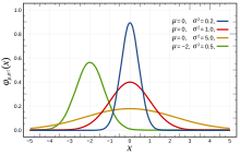
In probability theory and statistics, a probability distribution is the mathematical function that gives the probabilities of occurrence of different possible outcomes for an experiment. It is a mathematical description of a random phenomenon in terms of its sample space and the probabilities of events.

<span class="mw-page-title-main">Skewness</span> Measure of the asymmetry of random variables

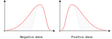
In probability theory and statistics, skewness is a measure of the asymmetry of the probability distribution of a real-valued random variable about its mean. The skewness value can be positive, zero, negative, or undefined.

In statistics, the mean squared error (MSE) or mean squared deviation (MSD) of an estimator measures the average of the squares of the errors—that is, the average squared difference between the estimated values and the actual value. MSE is a risk function, corresponding to the expected value of the squared error loss. The fact that MSE is almost always strictly positive is because of randomness or because the estimator does not account for information that could produce a more accurate estimate. In machine learning, specifically empirical risk minimization, MSE may refer to the empirical risk, as an estimate of the true MSE.

<span class="mw-page-title-main">Weibull distribution</span> Continuous probability distribution

In probability theory and statistics, the Weibull distribution is a continuous probability distribution. It models a broad range of random variables, largely in the nature of a time to failure or time between events. Examples are maximum one-day rainfalls and the time a user spends on a web page.

<span class="mw-page-title-main">Gamma distribution</span> Probability distribution

In probability theory and statistics, the gamma distribution is a versatile two-parameter family of continuous probability distributions. The exponential distribution, Erlang distribution, and chi-squared distribution are special cases of the gamma distribution. There are two equivalent parameterizations in common use:

  1. With a shape parameter k and a scale parameter θ
  2. With a shape parameter and an inverse scale parameter , called a rate parameter.

In probability and statistics, an exponential family is a parametric set of probability distributions of a certain form, specified below. This special form is chosen for mathematical convenience, including the enabling of the user to calculate expectations, covariances using differentiation based on some useful algebraic properties, as well as for generality, as exponential families are in a sense very natural sets of distributions to consider. The term exponential class is sometimes used in place of "exponential family", or the older term Koopman–Darmois family. Sometimes loosely referred to as "the" exponential family, this class of distributions is distinct because they all possess a variety of desirable properties, most importantly the existence of a sufficient statistic.

In mathematical statistics, the Fisher information is a way of measuring the amount of information that an observable random variable X carries about an unknown parameter θ of a distribution that models X. Formally, it is the variance of the score, or the expected value of the observed information.

In statistics, a generalized linear model (GLM) is a flexible generalization of ordinary linear regression. The GLM generalizes linear regression by allowing the linear model to be related to the response variable via a link function and by allowing the magnitude of the variance of each measurement to be a function of its predicted value.

<span class="mw-page-title-main">Consistent estimator</span> Statistical estimator converging in probability to a true parameter as sample size increases

In statistics, a consistent estimator or asymptotically consistent estimator is an estimator—a rule for computing estimates of a parameter θ0—having the property that as the number of data points used increases indefinitely, the resulting sequence of estimates converges in probability to θ0. This means that the distributions of the estimates become more and more concentrated near the true value of the parameter being estimated, so that the probability of the estimator being arbitrarily close to θ0 converges to one.

<span class="mw-page-title-main">Hyperbolic secant distribution</span> Continuous probability distribution

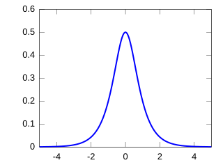
In probability theory and statistics, the hyperbolic secant distribution is a continuous probability distribution whose probability density function and characteristic function are proportional to the hyperbolic secant function. The hyperbolic secant function is equivalent to the reciprocal hyperbolic cosine, and thus this distribution is also called the inverse-cosh distribution.

In statistics, Poisson regression is a generalized linear model form of regression analysis used to model count data and contingency tables. Poisson regression assumes the response variable Y has a Poisson distribution, and assumes the logarithm of its expected value can be modeled by a linear combination of unknown parameters. A Poisson regression model is sometimes known as a log-linear model, especially when used to model contingency tables.

In statistics, binomial regression is a regression analysis technique in which the response has a binomial distribution: it is the number of successes in a series of independent Bernoulli trials, where each trial has probability of success . In binomial regression, the probability of a success is related to explanatory variables: the corresponding concept in ordinary regression is to relate the mean value of the unobserved response to explanatory variables.

In the statistical area of survival analysis, an accelerated failure time model is a parametric model that provides an alternative to the commonly used proportional hazards models. Whereas a proportional hazards model assumes that the effect of a covariate is to multiply the hazard by some constant, an AFT model assumes that the effect of a covariate is to accelerate or decelerate the life course of a disease by some constant. There is strong basic science evidence from C. Elegans experiments by Stroustrup et al. indicating that AFT models are the correct model for biological survival processes.

In statistics, efficiency is a measure of quality of an estimator, of an experimental design, or of a hypothesis testing procedure. Essentially, a more efficient estimator needs fewer input data or observations than a less efficient one to achieve the Cramér–Rao bound. An efficient estimator is characterized by having the smallest possible variance, indicating that there is a small deviance between the estimated value and the "true" value in the L2 norm sense.

<span class="mw-page-title-main">CumFreq</span> Software tool for data analysis and statistics

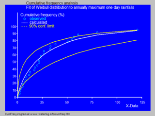
In statistics and data analysis the application software CumFreq is a tool for cumulative frequency analysis of a single variable and for probability distribution fitting.

<span class="mw-page-title-main">Beta rectangular distribution</span>

In probability theory and statistics, the beta rectangular distribution is a probability distribution that is a finite mixture distribution of the beta distribution and the continuous uniform distribution. The support is of the distribution is indicated by the parameters a and b, which are the minimum and maximum values respectively. The distribution provides an alternative to the beta distribution such that it allows more density to be placed at the extremes of the bounded interval of support. Thus it is a bounded distribution that allows for outliers to have a greater chance of occurring than does the beta distribution.

<span class="mw-page-title-main">Hermite distribution</span> Statistical probability Distribution for discrete event counts

In probability theory and statistics, the Hermite distribution, named after Charles Hermite, is a discrete probability distribution used to model count data with more than one parameter. This distribution is flexible in terms of its ability to allow a moderate over-dispersion in the data.

<span class="mw-page-title-main">Cumulative frequency analysis</span>

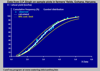
Cumulative frequency analysis is the analysis of the frequency of occurrence of values of a phenomenon less than a reference value. The phenomenon may be time- or space-dependent. Cumulative frequency is also called frequency of non-exceedance.

In statistics, the class of vector generalized linear models (VGLMs) was proposed to enlarge the scope of models catered for by generalized linear models (GLMs). In particular, VGLMs allow for response variables outside the classical exponential family and for more than one parameter. Each parameter can be transformed by a link function. The VGLM framework is also large enough to naturally accommodate multiple responses; these are several independent responses each coming from a particular statistical distribution with possibly different parameter values.

References

  1. 1 2 Left (negatively) skewed frequency histograms can be fitted to square Normal or mirrored Gumbel probability functions. On line:
  2. Frequency and Regression Analysis. Chapter 6 in: H.P.Ritzema (ed., 1994), Drainage Principles and Applications, Publ. 16, pp. 175–224, International Institute for Land Reclamation and Improvement (ILRI), Wageningen, The Netherlands. ISBN   9070754339. Free download from the webpage under nr. 12, or directly as PDF :
  3. H. Cramér, "Mathematical methods of statistics", Princeton Univ. Press (1946)
  4. Hosking, J.R.M. (1990). "L-moments: analysis and estimation of distributions using linear combinations of order statistics". Journal of the Royal Statistical Society, Series B. 52 (1): 105–124. JSTOR   2345653.
  5. Aldrich, John (1997). "R. A. Fisher and the making of maximum likelihood 1912–1922". Statistical Science. 12 (3): 162–176. doi: 10.1214/ss/1030037906 . MR   1617519.
  6. 1 2 3 Software for Generalized and Composite Probability Distributions. International Journal of Mathematical and Computational Methods, 4, 1-9 or
  7. Example of an approximately normally distributed data set to which a large number of different probability distributions can be fitted,
  8. Left (negatively) skewed frequency histograms can be fitted to square normal or mirrored Gumbel probability functions.
  9. Intro to composite probability distributions
  10. Frequency predictions and their binomial confidence limits. In: International Commission on Irrigation and Drainage, Special Technical Session: Economic Aspects of Flood Control and non-Structural Measures, Dubrovnik, Yugoslavia, 1988. On line
  11. Benson, M.A. 1960. Characteristics of frequency curves based on a theoretical 1000 year record. In: T.Dalrymple (Ed.), Flood frequency analysis. U.S. Geological Survey Water Supply Paper, 1543-A, pp. 51-71.
  12. Pijlman; Linnartz (2023). "Variance of Likelihood of data". SITB 2023 Proceedings: 34.
  13. Software for probability distribution fitting