A histogram is an approximate representation of the distribution of numerical data. It was first introduced by Karl Pearson. To construct a histogram, the first step is to "bin" the range of values—that is, divide the entire range of values into a series of intervals—and then count how many values fall into each interval. The bins are usually specified as consecutive, non-overlapping intervals of a variable. The bins (intervals) must be adjacent and are often of equal size.

In probability theory, a normaldistribution is a type of continuous probability distribution for a real-valued random variable. The general form of its probability density function is

In probability theory and statistics, skewness is a measure of the asymmetry of the probability distribution of a real-valued random variable about its mean. The skewness value can be positive, zero, negative, or undefined.

In statistics, rankits of a set of data are the expected values of the order statistics of a sample from the standard normal distribution the same size as the data. They are primarily used in the normal probability plot, a graphical technique for normality testing.

In statistics, a bimodaldistribution is a probability distribution with two different modes, which may also be referred to as a bimodal distribution. These appear as distinct peaks in the probability density function, as shown in Figures 1 and 2. Categorical, continuous, and discrete data can all form bimodal distributions.
The mode is the value that appears most often in a set of data values. If X is a discrete random variable, the mode is the value x at which the probability mass function takes its maximum value. In other words, it is the value that is most likely to be sampled.
In mathematics, unimodality means possessing a unique mode. More generally, unimodality means there is only a single highest value, somehow defined, of some mathematical object.

In probability theory and statistics, the probit function is the quantile function associated with the standard normal distribution. It has applications in data analysis and machine learning, in particular exploratory statistical graphics and specialized regression modeling of binary response variables.
The following is a glossary of terms used in the mathematical sciences statistics and probability.

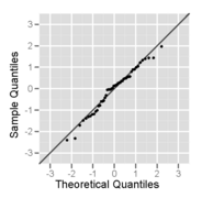
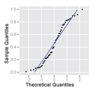
In statistics, a Q–Q (quantile-quantile) plot is a probability plot, which is a graphical method for comparing two probability distributions by plotting their quantiles against each other. First, the set of intervals for the quantiles is chosen. A point (x, y) on the plot corresponds to one of the quantiles of the second distribution plotted against the same quantile of the first distribution. Thus the line is a parametric curve with the parameter which is the number of the interval for the quantile.
In statistics, normality tests are used to determine if a data set is well-modeled by a normal distribution and to compute how likely it is for a random variable underlying the data set to be normally distributed.
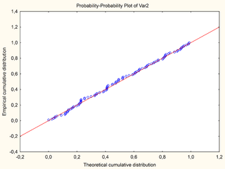
In statistics, a P–P plot is a probability plot for assessing how closely two data sets agree, which plots the two cumulative distribution functions against each other. P-P plots are vastly used to evaluate the skewness of a distribution.
In probability and statistics, the quantile function, associated with a probability distribution of a random variable, specifies the value of the random variable such that the probability of the variable being less than or equal to that value equals the given probability. It is also called the percent-point function or inverse cumulative distribution function.
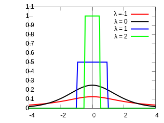
Formalized by John Tukey, the Tukey lambda distribution is a continuous, symmetric probability distribution defined in terms of its quantile function. It is typically used to identify an appropriate distribution and not used in statistical models directly.

In probability theory and statistics, the skew normal distribution is a continuous probability distribution that generalises the normal distribution to allow for non-zero skewness.
In statistics and probability theory, the nonparametric skew is a statistic occasionally used with random variables that take real values. It is a measure of the skewness of a random variable's distribution—that is, the distribution's tendency to "lean" to one side or the other of the mean. Its calculation does not require any knowledge of the form of the underlying distribution—hence the name nonparametric. It has some desirable properties: it is zero for any symmetric distribution; it is unaffected by a scale shift; and it reveals either left- or right-skewness equally well. In some statistical samples it has been shown to be less powerful than the usual measures of skewness in detecting departures of the population from normality.
In statistics, a symmetric probability distribution is a probability distribution—an assignment of probabilities to possible occurrences—which is unchanged when its probability density function or probability mass function is reflected around a vertical line at some value of the random variable represented by the distribution. This vertical line is the line of symmetry of the distribution. Thus the probability of being any given distance on one side of the value about which symmetry occurs is the same as the probability of being the same distance on the other side of that value.
Quantile-parameterized distributions (QPDs) are probability distributions that are directly parameterized by data. They were motivated by the need for easy-to-use continuous probability distributions flexible enough to represent a wide range of uncertainties, such as those commonly encountered in business, economics, engineering, and science. Because QPDs are directly parameterized by data, they have the practical advantage of avoiding the intermediate step of parameter estimation, a time-consuming process that typically requires non-linear iterative methods to estimate probability-distribution parameters from data. Some QPDs have virtually unlimited shape flexibility and closed-form moments as well.