Nonlinear regression

Last updated March 28, 2024

In statistics, nonlinear regression is a form of regression analysis in which observational data are modeled by a function which is a nonlinear combination of the model parameters and depends on one or more independent variables. The data are fitted by a method of successive approximations (iterations).

General

In nonlinear regression, a statistical model of the form,

\mathbf {y} \sim f(\mathbf {x} ,{\boldsymbol {\beta }})

relates a vector of independent variables, $\mathbf {x}$ , and its associated observed dependent variables, $\mathbf {y}$ . The function $f$ is nonlinear in the components of the vector of parameters $\beta$ , but otherwise arbitrary. For example, the Michaelis–Menten model for enzyme kinetics has two parameters and one independent variable, related by $f$ by:^{[lower-alpha 1]}

f(x,{\boldsymbol {\beta }})={\frac {\beta _{1}x}{\beta _{2}+x}}

This function, which is a rectangular hyperbola, is nonlinear because it cannot be expressed as a linear combination of the two $\beta$ s.

Systematic error may be present in the independent variables but its treatment is outside the scope of regression analysis. If the independent variables are not error-free, this is an errors-in-variables model, also outside this scope.

Other examples of nonlinear functions include exponential functions, logarithmic functions, trigonometric functions, power functions, Gaussian function, and Lorentz distributions. Some functions, such as the exponential or logarithmic functions, can be transformed so that they are linear. When so transformed, standard linear regression can be performed but must be applied with caution. See Linearization§Transformation, below, for more details.

In general, there is no closed-form expression for the best-fitting parameters, as there is in linear regression. Usually numerical optimization algorithms are applied to determine the best-fitting parameters. Again in contrast to linear regression, there may be many local minima of the function to be optimized and even the global minimum may produce a biased estimate. In practice, estimated values of the parameters are used, in conjunction with the optimization algorithm, to attempt to find the global minimum of a sum of squares.

For details concerning nonlinear data modeling see least squares and non-linear least squares.

Regression statistics

The assumption underlying this procedure is that the model can be approximated by a linear function, namely a first-order Taylor series:

f(x_{i},{\boldsymbol {\beta }})\approx f(x_{i},0)+\sum _{j}J_{ij}\beta _{j}

where $J_{ij}={\frac {\partial f(x_{i},{\boldsymbol {\beta }})}{\partial \beta _{j}}}$ are Jacobian matrix elements. It follows from this that the least squares estimators are given by

{\hat {\boldsymbol {\beta }}}\approx \mathbf {(J^{T}J)^{-1}J^{T}y} ,

compare generalized least squares with covariance matrix proportional to the unit matrix. The nonlinear regression statistics are computed and used as in linear regression statistics, but using J in place of X in the formulas.

When the function $f(x_{i},{\boldsymbol {\beta }})$ itself is not known analytically, but needs to be linearly approximated from $n+1$ , or more, known values (where $n$ is the number of estimators), the best estimator is obtained directly from the Linear Template Fit as ^[1]

{\hat {\boldsymbol {\beta }}}=((\mathbf {Y{\tilde {M}}} )^{\mathsf {T}}{\boldsymbol {\Omega }}^{-1}\mathbf {Y{\tilde {M}}} )^{-1}(\mathbf {Y{\tilde {M}}} )^{\mathsf {T}}{\boldsymbol {\Omega }}^{-1}(\mathbf {d} -\mathbf {Y{\bar {m}})}

(see also linear least squares).

The linear approximation introduces bias into the statistics. Therefore, more caution than usual is required in interpreting statistics derived from a nonlinear model.

Ordinary and weighted least squares

The best-fit curve is often assumed to be that which minimizes the sum of squared residuals. This is the ordinary least squares (OLS) approach. However, in cases where the dependent variable does not have constant variance, or there are some outliers, a sum of weighted squared residuals may be minimized; see weighted least squares. Each weight should ideally be equal to the reciprocal of the variance of the observation, or the reciprocal of the dependent variable to some power in the outlier case ^[2] , but weights may be recomputed on each iteration, in an iteratively weighted least squares algorithm.

Linearization

Transformation

Some nonlinear regression problems can be moved to a linear domain by a suitable transformation of the model formulation.

For example, consider the nonlinear regression problem

y=ae^{bx}U\,\!

with parameters a and b and with multiplicative error term U. If we take the logarithm of both sides, this becomes

\ln {(y)}=\ln {(a)}+bx+u,\,\!

where u = ln(U), suggesting estimation of the unknown parameters by a linear regression of ln(y) on x, a computation that does not require iterative optimization. However, use of a nonlinear transformation requires caution. The influences of the data values will change, as will the error structure of the model and the interpretation of any inferential results. These may not be desired effects. On the other hand, depending on what the largest source of error is, a nonlinear transformation may distribute the errors in a Gaussian fashion, so the choice to perform a nonlinear transformation must be informed by modeling considerations.

For Michaelis–Menten kinetics, the linear Lineweaver–Burk plot

{\frac {1}{v}}={\frac {1}{V_{\max }}}+{\frac {K_{m}}{V_{\max }[S]}}

of 1/v against 1/[S] has been much used. However, since it is very sensitive to data error and is strongly biased toward fitting the data in a particular range of the independent variable, [S], its use is strongly discouraged.

For error distributions that belong to the exponential family, a link function may be used to transform the parameters under the Generalized linear model framework.

Segmentation

The independent or explanatory variable (say X) can be split up into classes or segments and linear regression can be performed per segment. Segmented regression with confidence analysis may yield the result that the dependent or response variable (say Y) behaves differently in the various segments.^[3]

The figure shows that the soil salinity (X) initially exerts no influence on the crop yield (Y) of mustard, until a critical or threshold value (breakpoint), after which the yield is affected negatively.^[4]

Related Research Articles

The method of least squares is a parameter estimation method in regression analysis based on minimizing the sum of the squares of the residuals made in the results of each individual equation.

In statistics, the Gauss–Markov theorem states that the ordinary least squares (OLS) estimator has the lowest sampling variance within the class of linear unbiased estimators, if the errors in the linear regression model are uncorrelated, have equal variances and expectation value of zero. The errors do not need to be normal for the theorem to apply, nor do they need to be independent and identically distributed.

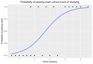
In statistics, the logistic model is a statistical model that models the log-odds of an event as a linear combination of one or more independent variables. In regression analysis, logistic regression is estimating the parameters of a logistic model. Formally, in binary logistic regression there is a single binary dependent variable, coded by an indicator variable, where the two values are labeled "0" and "1", while the independent variables can each be a binary variable or a continuous variable. The corresponding probability of the value labeled "1" can vary between 0 and 1, hence the labeling; the function that converts log-odds to probability is the logistic function, hence the name. The unit of measurement for the log-odds scale is called a logit, from logistic unit, hence the alternative names. See § Background and § Definition for formal mathematics, and § Example for a worked example.

In statistics, a generalized linear model (GLM) is a flexible generalization of ordinary linear regression. The GLM generalizes linear regression by allowing the linear model to be related to the response variable via a link function and by allowing the magnitude of the variance of each measurement to be a function of its predicted value.

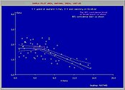
In statistical modeling, regression analysis is a set of statistical processes for estimating the relationships between a dependent variable and one or more independent variables. The most common form of regression analysis is linear regression, in which one finds the line that most closely fits the data according to a specific mathematical criterion. For example, the method of ordinary least squares computes the unique line that minimizes the sum of squared differences between the true data and that line. For specific mathematical reasons, this allows the researcher to estimate the conditional expectation of the dependent variable when the independent variables take on a given set of values. Less common forms of regression use slightly different procedures to estimate alternative location parameters or estimate the conditional expectation across a broader collection of non-linear models.

In mathematics and computing, the Levenberg–Marquardt algorithm, also known as the damped least-squares (DLS) method, is used to solve non-linear least squares problems. These minimization problems arise especially in least squares curve fitting. The LMA interpolates between the Gauss–Newton algorithm (GNA) and the method of gradient descent. The LMA is more robust than the GNA, which means that in many cases it finds a solution even if it starts very far off the final minimum. For well-behaved functions and reasonable starting parameters, the LMA tends to be slower than the GNA. LMA can also be viewed as Gauss–Newton using a trust region approach.

In applied statistics, total least squares is a type of errors-in-variables regression, a least squares data modeling technique in which observational errors on both dependent and independent variables are taken into account. It is a generalization of Deming regression and also of orthogonal regression, and can be applied to both linear and non-linear models.

The Gauss–Newton algorithm is used to solve non-linear least squares problems, which is equivalent to minimizing a sum of squared function values. It is an extension of Newton's method for finding a minimum of a non-linear function. Since a sum of squares must be nonnegative, the algorithm can be viewed as using Newton's method to iteratively approximate zeroes of the components of the sum, and thus minimizing the sum. In this sense, the algorithm is also an effective method for solving overdetermined systems of equations. It has the advantage that second derivatives, which can be challenging to compute, are not required.

In statistics, ordinary least squares (OLS) is a type of linear least squares method for choosing the unknown parameters in a linear regression model by the principle of least squares: minimizing the sum of the squares of the differences between the observed dependent variable in the input dataset and the output of the (linear) function of the independent variable.

Weighted least squares (WLS), also known as weighted linear regression, is a generalization of ordinary least squares and linear regression in which knowledge of the unequal variance of observations (heteroscedasticity) is incorporated into the regression. WLS is also a specialization of generalized least squares, when all the off-diagonal entries of the covariance matrix of the errors, are null.

In statistics, multinomial logistic regression is a classification method that generalizes logistic regression to multiclass problems, i.e. with more than two possible discrete outcomes. That is, it is a model that is used to predict the probabilities of the different possible outcomes of a categorically distributed dependent variable, given a set of independent variables.

In statistics, generalized least squares (GLS) is a method used to estimate the unknown parameters in a linear regression model. It is used when there is a non-zero amount of correlation between the residuals in the regression model. GLS is employed to improve statistical efficiency and reduce the risk of drawing erroneous inferences, as compared to conventional least squares and weighted least squares methods. It was first described by Alexander Aitken in 1935.

In statistics, binomial regression is a regression analysis technique in which the response has a binomial distribution: it is the number of successes in a series of independent Bernoulli trials, where each trial has probability of success . In binomial regression, the probability of a success is related to explanatory variables: the corresponding concept in ordinary regression is to relate the mean value of the unobserved response to explanatory variables.

Bayesian linear regression is a type of conditional modeling in which the mean of one variable is described by a linear combination of other variables, with the goal of obtaining the posterior probability of the regression coefficients and ultimately allowing the out-of-sample prediction of the regressandconditional on observed values of the regressors. The simplest and most widely used version of this model is the normal linear model, in which $given is distributed Gaussian. In this model, and under a particular choice of prior probabilities for the parameters—so-called conjugate priors—the posterior can be found analytically. With more arbitrarily chosen priors, the posteriors generally have to be approximated.$

The topic of heteroskedasticity-consistent (HC) standard errors arises in statistics and econometrics in the context of linear regression and time series analysis. These are also known as heteroskedasticity-robust standard errors, Eicker–Huber–White standard errors, to recognize the contributions of Friedhelm Eicker, Peter J. Huber, and Halbert White.

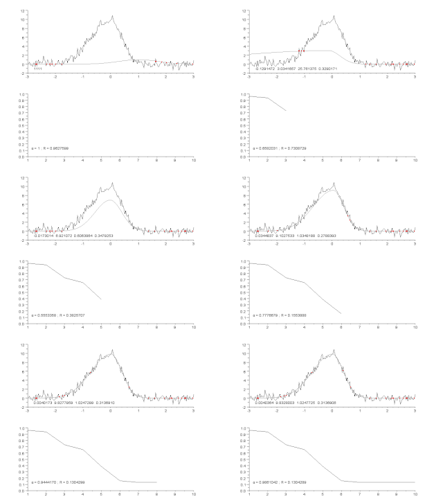
Non-linear least squares is the form of least squares analysis used to fit a set of m observations with a model that is non-linear in n unknown parameters (m ≥ n). It is used in some forms of nonlinear regression. The basis of the method is to approximate the model by a linear one and to refine the parameters by successive iterations. There are many similarities to linear least squares, but also some significant differences. In economic theory, the non-linear least squares method is applied in (i) the probit regression, (ii) threshold regression, (iii) smooth regression, (iv) logistic link regression, (v) Box–Cox transformed regressors ( $).$

In statistics, principal component regression (PCR) is a regression analysis technique that is based on principal component analysis (PCA). More specifically, PCR is used for estimating the unknown regression coefficients in a standard linear regression model.

Linear least squares (LLS) is the least squares approximation of linear functions to data. It is a set of formulations for solving statistical problems involved in linear regression, including variants for ordinary (unweighted), weighted, and generalized (correlated) residuals. Numerical methods for linear least squares include inverting the matrix of the normal equations and orthogonal decomposition methods.

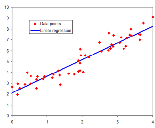
In statistics, linear regression is a statistical model which estimates the linear relationship between a scalar response and one or more explanatory variables. The case of one explanatory variable is called simple linear regression; for more than one, the process is called multiple linear regression. This term is distinct from multivariate linear regression, where multiple correlated dependent variables are predicted, rather than a single scalar variable. If the explanatory variables are measured with error then errors-in-variables models are required, also known as measurement error models.

In statistics, the class of vector generalized linear models (VGLMs) was proposed to enlarge the scope of models catered for by generalized linear models (GLMs). In particular, VGLMs allow for response variables outside the classical exponential family and for more than one parameter. Each parameter can be transformed by a link function. The VGLM framework is also large enough to naturally accommodate multiple responses; these are several independent responses each coming from a particular statistical distribution with possibly different parameter values.

References

↑ Britzger, Daniel (2022). "The Linear Template Fit". Eur. Phys. J. C. 82 (8): 731. arXiv: 2112.01548 . Bibcode:2022EPJC...82..731B. doi:10.1140/epjc/s10052-022-10581-w.
↑ Motulsky, H.J.; Ransnas, L.A. (1987). "Fitting curves to data using nonlinear regression: a practical and nonmathematical review". The FASEB Journal. 1 (5): 365–374. doi: 10.1096/fasebj.1.5.3315805 . PMID 3315805.
↑ R.J.Oosterbaan, 1994, Frequency and Regression Analysis. In: H.P.Ritzema (ed.), Drainage Principles and Applications, Publ. 16, pp. 175-224, International Institute for Land Reclamation and Improvement (ILRI), Wageningen, The Netherlands. ISBN 90-70754-33-9 . Download as PDF :
↑ R.J.Oosterbaan, 2002. Drainage research in farmers' fields: analysis of data. Part of project “Liquid Gold” of the International Institute for Land Reclamation and Improvement (ILRI), Wageningen, The Netherlands. Download as PDF : . The figure was made with the SegReg program, which can be downloaded freely from

Notes

↑ This model can also be expressed in the conventional biological notation:
$v={\frac {V_{\max }\ [{\mbox{S}}]}{K_{m}+[{\mbox{S}}]}}$