In statistics, the term linear model refers to any model which assumes linearity in the system. The most common occurrence is in connection with regression models and the term is often taken as synonymous with linear regression model. However, the term is also used in time series analysis with a different meaning. In each case, the designation "linear" is used to identify a subclass of models for which substantial reduction in the complexity of the related statistical theory is possible.
In statistics, the Gauss–Markov theorem states that the ordinary least squares (OLS) estimator has the lowest sampling variance within the class of linear unbiased estimators, if the errors in the linear regression model are uncorrelated, have equal variances and expectation value of zero. The errors do not need to be normal for the theorem to apply, nor do they need to be independent and identically distributed.
Levinson recursion or Levinson–Durbin recursion is a procedure in linear algebra to recursively calculate the solution to an equation involving a Toeplitz matrix. The algorithm runs in Θ(n2) time, which is a strong improvement over Gauss–Jordan elimination, which runs in Θ(n3).

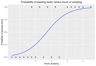
In statistics, the logistic model is a statistical model that models the log-odds of an event as a linear combination of one or more independent variables. In regression analysis, logistic regression is estimating the parameters of a logistic model. Formally, in binary logistic regression there is a single binary dependent variable, coded by an indicator variable, where the two values are labeled "0" and "1", while the independent variables can each be a binary variable or a continuous variable. The corresponding probability of the value labeled "1" can vary between 0 and 1, hence the labeling; the function that converts log-odds to probability is the logistic function, hence the name. The unit of measurement for the log-odds scale is called a logit, from logistic unit, hence the alternative names. See § Background and § Definition for formal mathematics, and § Example for a worked example.

In statistics, originally in geostatistics, kriging or Kriging, also known as Gaussian process regression, is a method of interpolation based on Gaussian process governed by prior covariances. Under suitable assumptions of the prior, kriging gives the best linear unbiased prediction (BLUP) at unsampled locations. Interpolating methods based on other criteria such as smoothness may not yield the BLUP. The method is widely used in the domain of spatial analysis and computer experiments. The technique is also known as Wiener–Kolmogorov prediction, after Norbert Wiener and Andrey Kolmogorov.

In statistical modeling, regression analysis is a set of statistical processes for estimating the relationships between a dependent variable and one or more independent variables. The most common form of regression analysis is linear regression, in which one finds the line that most closely fits the data according to a specific mathematical criterion. For example, the method of ordinary least squares computes the unique line that minimizes the sum of squared differences between the true data and that line. For specific mathematical reasons, this allows the researcher to estimate the conditional expectation of the dependent variable when the independent variables take on a given set of values. Less common forms of regression use slightly different procedures to estimate alternative location parameters or estimate the conditional expectation across a broader collection of non-linear models.
In statistics and in particular in regression analysis, a design matrix, also known as model matrix or regressor matrix and often denoted by X, is a matrix of values of explanatory variables of a set of objects. Each row represents an individual object, with the successive columns corresponding to the variables and their specific values for that object. The design matrix is used in certain statistical models, e.g., the general linear model. It can contain indicator variables that indicate group membership in an ANOVA, or it can contain values of continuous variables.
In statistics, ordinary least squares (OLS) is a type of linear least squares method for choosing the unknown parameters in a linear regression model by the principle of least squares: minimizing the sum of the squares of the differences between the observed dependent variable in the input dataset and the output of the (linear) function of the independent variable.

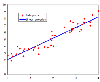
In statistics, simple linear regression (SLR) is a linear regression model with a single explanatory variable. That is, it concerns two-dimensional sample points with one independent variable and one dependent variable and finds a linear function that, as accurately as possible, predicts the dependent variable values as a function of the independent variable. The adjective simple refers to the fact that the outcome variable is related to a single predictor.
In statistics, multinomial logistic regression is a classification method that generalizes logistic regression to multiclass problems, i.e. with more than two possible discrete outcomes. That is, it is a model that is used to predict the probabilities of the different possible outcomes of a categorically distributed dependent variable, given a set of independent variables.
In statistics, generalized least squares (GLS) is a method used to estimate the unknown parameters in a linear regression model. It is used when there is a non-zero amount of correlation between the residuals in the regression model. GLS is employed to improve statistical efficiency and reduce the risk of drawing erroneous inferences, as compared to conventional least squares and weighted least squares methods. It was first described by Alexander Aitken in 1935.
In mathematics, a moment matrix is a special symmetric square matrix whose rows and columns are indexed by monomials. The entries of the matrix depend on the product of the indexing monomials only
In statistics, Bayesian multivariate linear regression is a Bayesian approach to multivariate linear regression, i.e. linear regression where the predicted outcome is a vector of correlated random variables rather than a single scalar random variable. A more general treatment of this approach can be found in the article MMSE estimator.
In statistics and econometrics, the multivariate probit model is a generalization of the probit model used to estimate several correlated binary outcomes jointly. For example, if it is believed that the decisions of sending at least one child to public school and that of voting in favor of a school budget are correlated, then the multivariate probit model would be appropriate for jointly predicting these two choices on an individual-specific basis. J.R. Ashford and R.R. Sowden initially proposed an approach for multivariate probit analysis. Siddhartha Chib and Edward Greenberg extended this idea and also proposed simulation-based inference methods for the multivariate probit model which simplified and generalized parameter estimation.
Linear least squares (LLS) is the least squares approximation of linear functions to data. It is a set of formulations for solving statistical problems involved in linear regression, including variants for ordinary (unweighted), weighted, and generalized (correlated) residuals. Numerical methods for linear least squares include inverting the matrix of the normal equations and orthogonal decomposition methods.
In econometrics, Prais–Winsten estimation is a procedure meant to take care of the serial correlation of type AR(1) in a linear model. Conceived by Sigbert Prais and Christopher Winsten in 1954, it is a modification of Cochrane–Orcutt estimation in the sense that it does not lose the first observation, which leads to more efficiency as a result and makes it a special case of feasible generalized least squares.
In statistics and in machine learning, a linear predictor function is a linear function of a set of coefficients and explanatory variables, whose value is used to predict the outcome of a dependent variable. This sort of function usually comes in linear regression, where the coefficients are called regression coefficients. However, they also occur in various types of linear classifiers, as well as in various other models, such as principal component analysis and factor analysis. In many of these models, the coefficients are referred to as "weights".
In statistics, linear regression is a statistical model which estimates the linear relationship between a scalar response and one or more explanatory variables. The case of one explanatory variable is called simple linear regression; for more than one, the process is called multiple linear regression. This term is distinct from multivariate linear regression, where multiple correlated dependent variables are predicted, rather than a single scalar variable. If the explanatory variables are measured with error then errors-in-variables models are required, also known as measurement error models.
In statistics, particularly regression analysis, the Working–Hotelling procedure, named after Holbrook Working and Harold Hotelling, is a method of simultaneous estimation in linear regression models. One of the first developments in simultaneous inference, it was devised by Working and Hotelling for the simple linear regression model in 1929. It provides a confidence region for multiple mean responses, that is, it gives the upper and lower bounds of more than one value of a dependent variable at several levels of the independent variables at a certain confidence level. The resulting confidence bands are known as the Working–Hotelling–Scheffé confidence bands.
Functional regression is a version of regression analysis when responses or covariates include functional data. Functional regression models can be classified into four types depending on whether the responses or covariates are functional or scalar: (i) scalar responses with functional covariates, (ii) functional responses with scalar covariates, (iii) functional responses with functional covariates, and (iv) scalar or functional responses with functional and scalar covariates. In addition, functional regression models can be linear, partially linear, or nonlinear. In particular, functional polynomial models, functional single and multiple index models and functional additive models are three special cases of functional nonlinear models.


