In analytic geometry, an asymptote of a curve is a line such that the distance between the curve and the line approaches zero as one or both of the x or y coordinates tends to infinity. In projective geometry and related contexts, an asymptote of a curve is a line which is tangent to the curve at a point at infinity.

In the mathematical field of numerical analysis, interpolation is a type of estimation, a method of constructing (finding) new data points based on the range of a discrete set of known data points.
In mathematics, a polynomial is an expression consisting of indeterminates and coefficients, that involves only the operations of addition, subtraction, multiplication, and non-negative integer exponentiation of variables. An example of a polynomial of a single indeterminate x is x2 − 4x + 7. An example in three variables is x3 + 2xyz2 − yz + 1.

In mathematics, an affine algebraic plane curve is the zero set of a polynomial in two variables. A projective algebraic plane curve is the zero set in a projective plane of a homogeneous polynomial in three variables. An affine algebraic plane curve can be completed in a projective algebraic plane curve by homogenizing its defining polynomial. Conversely, a projective algebraic plane curve of homogeneous equation h(x, y, t) = 0 can be restricted to the affine algebraic plane curve of equation h(x, y, 1) = 0. These two operations are each inverse to the other; therefore, the phrase algebraic plane curve is often used without specifying explicitly whether it is the affine or the projective case that is considered.
In mathematics, a quadratic irrational number is an irrational number that is the solution to some quadratic equation with rational coefficients which is irreducible over the rational numbers. Since fractions in the coefficients of a quadratic equation can be cleared by multiplying both sides by their least common denominator, a quadratic irrational is an irrational root of some quadratic equation with integer coefficients. The quadratic irrational numbers, a subset of the complex numbers, are algebraic numbers of degree 2, and can therefore be expressed as
In mathematics, a rational function is any function that can be defined by a rational fraction, which is an algebraic fraction such that both the numerator and the denominator are polynomials. The coefficients of the polynomials need not be rational numbers; they may be taken in any field K. In this case, one speaks of a rational function and a rational fraction over K. The values of the variables may be taken in any field L containing K. Then the domain of the function is the set of the values of the variables for which the denominator is not zero, and the codomain is L.

In control theory and stability theory, root locus analysis is a graphical method for examining how the roots of a system change with variation of a certain system parameter, commonly a gain within a feedback system. This is a technique used as a stability criterion in the field of classical control theory developed by Walter R. Evans which can determine stability of the system. The root locus plots the poles of the closed loop transfer function in the complex s-plane as a function of a gain parameter.

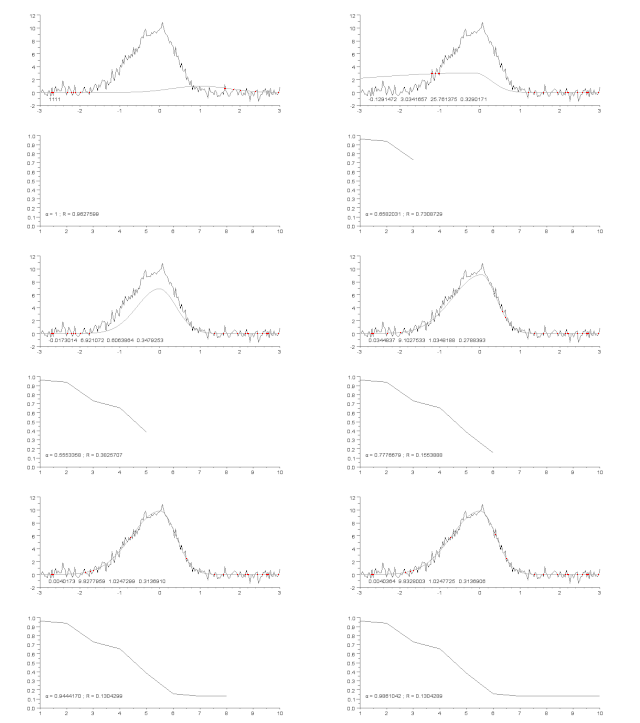
Curve fitting is the process of constructing a curve, or mathematical function, that has the best fit to a series of data points, possibly subject to constraints. Curve fitting can involve either interpolation, where an exact fit to the data is required, or smoothing, in which a "smooth" function is constructed that approximately fits the data. A related topic is regression analysis, which focuses more on questions of statistical inference such as how much uncertainty is present in a curve that is fit to data observed with random errors. Fitted curves can be used as an aid for data visualization, to infer values of a function where no data are available, and to summarize the relationships among two or more variables. Extrapolation refers to the use of a fitted curve beyond the range of the observed data, and is subject to a degree of uncertainty since it may reflect the method used to construct the curve as much as it reflects the observed data.

In mathematics, a square is the result of multiplying a number by itself. The verb "to square" is used to denote this operation. Squaring is the same as raising to the power 2, and is denoted by a superscript 2; for instance, the square of 3 may be written as 32, which is the number 9. In some cases when superscripts are not available, as for instance in programming languages or plain text files, the notations x^2 (caret) or x**2 may be used in place of x2. The adjective which corresponds to squaring is quadratic.
In statistics, ordinary least squares (OLS) is a type of linear least squares method for estimating the unknown parameters in a linear regression model. OLS chooses the parameters of a linear function of a set of explanatory variables by the principle of least squares: minimizing the sum of the squares of the differences between the observed dependent variable in the given dataset and those predicted by the linear function of the independent variable.
A height function is a function that quantifies the complexity of mathematical objects. In Diophantine geometry, height functions quantify the size of solutions to Diophantine equations and are typically functions from a set of points on algebraic varieties to the real numbers.
In mathematics, signal processing and control theory, a pole–zero plot is a graphical representation of a rational transfer function in the complex plane which helps to convey certain properties of the system such as:

Local regression or local polynomial regression, also known as moving regression, is a generalization of the moving average and polynomial regression. Its most common methods, initially developed for scatterplot smoothing, are LOESS and LOWESS, both pronounced. They are two strongly related non-parametric regression methods that combine multiple regression models in a k-nearest-neighbor-based meta-model. In some fields, LOESS is known and commonly referred to as Savitzky–Golay filter.

In statistics, response surface methodology (RSM) explores the relationships between several explanatory variables and one or more response variables. The method was introduced by George E. P. Box and K. B. Wilson in 1951. The main idea of RSM is to use a sequence of designed experiments to obtain an optimal response. Box and Wilson suggest using a second-degree polynomial model to do this. They acknowledge that this model is only an approximation, but they use it because such a model is easy to estimate and apply, even when little is known about the process.
In mathematics, a quadratic equation is a polynomial equation of the second degree. The general form is
In statistics, a sum of squares due to lack of fit, or more tersely a lack-of-fit sum of squares, is one of the components of a partition of the sum of squares of residuals in an analysis of variance, used in the numerator in an F-test of the null hypothesis that says that a proposed model fits well. The other component is the pure-error sum of squares.

In mathematics, a rational number is a number that can be expressed as the quotient or fraction p/q of two integers, a numerator p and a non-zero denominator q. For example, −3/7 is a rational number, as is every integer. The set of all rational numbers, also referred to as "the rationals", the field of rationals or the field of rational numbers is usually denoted by a boldface Q ; it was thus denoted in 1895 by Giuseppe Peano after quoziente, Italian for "quotient", and first appeared in Bourbaki's Algèbre.
In statistics, polynomial regression is a form of regression analysis in which the relationship between the independent variable x and the dependent variable y is modelled as an nth degree polynomial in x. Polynomial regression fits a nonlinear relationship between the value of x and the corresponding conditional mean of y, denoted E(y |x). Although polynomial regression fits a nonlinear model to the data, as a statistical estimation problem it is linear, in the sense that the regression function E(y | x) is linear in the unknown parameters that are estimated from the data. For this reason, polynomial regression is considered to be a special case of multiple linear regression.
Linear least squares (LLS) is the least squares approximation of linear functions to data. It is a set of formulations for solving statistical problems involved in linear regression, including variants for ordinary (unweighted), weighted, and generalized (correlated) residuals. Numerical methods for linear least squares include inverting the matrix of the normal equations and orthogonal decomposition methods.


