The likelihood function is the joint probability mass of observed data viewed as a function of the parameters of a statistical model. Intuitively, the likelihood function is the probability of observing data assuming is the actual parameter.
In statistics, maximum likelihood estimation (MLE) is a method of estimating the parameters of an assumed probability distribution, given some observed data. This is achieved by maximizing a likelihood function so that, under the assumed statistical model, the observed data is most probable. The point in the parameter space that maximizes the likelihood function is called the maximum likelihood estimate. The logic of maximum likelihood is both intuitive and flexible, and as such the method has become a dominant means of statistical inference.
In statistics, a statistic is sufficient with respect to a statistical model and its associated unknown parameter if "no other statistic that can be calculated from the same sample provides any additional information as to the value of the parameter". In particular, a statistic is sufficient for a family of probability distributions if the sample from which it is calculated gives no additional information than the statistic, as to which of those probability distributions is the sampling distribution.
In statistics, the mean squared error (MSE) or mean squared deviation (MSD) of an estimator measures the average of the squares of the errors—that is, the average squared difference between the estimated values and the actual value. MSE is a risk function, corresponding to the expected value of the squared error loss. The fact that MSE is almost always strictly positive is because of randomness or because the estimator does not account for information that could produce a more accurate estimate. In machine learning, specifically empirical risk minimization, MSE may refer to the empirical risk, as an estimate of the true MSE.

In probability theory and statistics, the gamma distribution is a versatile two-parameter family of continuous probability distributions. The exponential distribution, Erlang distribution, and chi-squared distribution are special cases of the gamma distribution. There are two equivalent parameterizations in common use:
- With a shape parameter k and a scale parameter θ
- With a shape parameter and an inverse scale parameter , called a rate parameter.
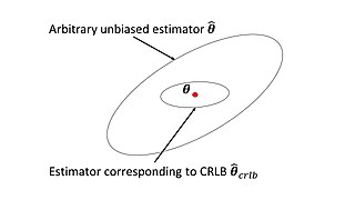
In estimation theory and statistics, the Cramér–Rao bound (CRB) relates to estimation of a deterministic parameter. The result is named in honor of Harald Cramér and C. R. Rao, but has also been derived independently by Maurice Fréchet, Georges Darmois, and by Alexander Aitken and Harold Silverstone. It is also known as Fréchet-Cramér–Rao or Fréchet-Darmois-Cramér-Rao lower bound. It states that the precision of any unbiased estimator is at most the Fisher information; or (equivalently) the reciprocal of the Fisher information is a lower bound on its variance.
In mathematical statistics, the Fisher information is a way of measuring the amount of information that an observable random variable X carries about an unknown parameter θ of a distribution that models X. Formally, it is the variance of the score, or the expected value of the observed information.
In statistics, sometimes the covariance matrix of a multivariate random variable is not known but has to be estimated. Estimation of covariance matrices then deals with the question of how to approximate the actual covariance matrix on the basis of a sample from the multivariate distribution. Simple cases, where observations are complete, can be dealt with by using the sample covariance matrix. The sample covariance matrix (SCM) is an unbiased and efficient estimator of the covariance matrix if the space of covariance matrices is viewed as an extrinsic convex cone in Rp×p; however, measured using the intrinsic geometry of positive-definite matrices, the SCM is a biased and inefficient estimator. In addition, if the random variable has a normal distribution, the sample covariance matrix has a Wishart distribution and a slightly differently scaled version of it is the maximum likelihood estimate. Cases involving missing data, heteroscedasticity, or autocorrelated residuals require deeper considerations. Another issue is the robustness to outliers, to which sample covariance matrices are highly sensitive.
In statistics, the theory of minimum norm quadratic unbiased estimation (MINQUE) was developed by C. R. Rao. MINQUE is a theory alongside other estimation methods in estimation theory, such as the method of moments or maximum likelihood estimation. Similar to the theory of best linear unbiased estimation, MINQUE is specifically concerned with linear regression models. The method was originally conceived to estimate heteroscedastic error variance in multiple linear regression. MINQUE estimators also provide an alternative to maximum likelihood estimators or restricted maximum likelihood estimators for variance components in mixed effects models. MINQUE estimators are quadratic forms of the response variable and are used to estimate a linear function of the variances.
In statistics, ordinary least squares (OLS) is a type of linear least squares method for choosing the unknown parameters in a linear regression model by the principle of least squares: minimizing the sum of the squares of the differences between the observed dependent variable in the input dataset and the output of the (linear) function of the independent variable.

In probability theory and statistics, the continuous uniform distributions or rectangular distributions are a family of symmetric probability distributions. Such a distribution describes an experiment where there is an arbitrary outcome that lies between certain bounds. The bounds are defined by the parameters, and which are the minimum and maximum values. The interval can either be closed or open. Therefore, the distribution is often abbreviated where stands for uniform distribution. The difference between the bounds defines the interval length; all intervals of the same length on the distribution's support are equally probable. It is the maximum entropy probability distribution for a random variable under no constraint other than that it is contained in the distribution's support.
In Bayesian statistics, a maximum a posteriori probability (MAP) estimate is an estimate of an unknown quantity, that equals the mode of the posterior distribution. The MAP can be used to obtain a point estimate of an unobserved quantity on the basis of empirical data. It is closely related to the method of maximum likelihood (ML) estimation, but employs an augmented optimization objective which incorporates a prior distribution over the quantity one wants to estimate. MAP estimation can therefore be seen as a regularization of maximum likelihood estimation.
In statistics, the Bayesian information criterion (BIC) or Schwarz information criterion is a criterion for model selection among a finite set of models; models with lower BIC are generally preferred. It is based, in part, on the likelihood function and it is closely related to the Akaike information criterion (AIC).
The James–Stein estimator is a biased estimator of the mean, , of (possibly) correlated Gaussian distributed random variables with unknown means .
In statistics, M-estimators are a broad class of extremum estimators for which the objective function is a sample average. Both non-linear least squares and maximum likelihood estimation are special cases of M-estimators. The definition of M-estimators was motivated by robust statistics, which contributed new types of M-estimators. However, M-estimators are not inherently robust, as is clear from the fact that they include maximum likelihood estimators, which are in general not robust. The statistical procedure of evaluating an M-estimator on a data set is called M-estimation.
The cross-entropy (CE) method is a Monte Carlo method for importance sampling and optimization. It is applicable to both combinatorial and continuous problems, with either a static or noisy objective.
In statistics, the bias of an estimator is the difference between this estimator's expected value and the true value of the parameter being estimated. An estimator or decision rule with zero bias is called unbiased. In statistics, "bias" is an objective property of an estimator. Bias is a distinct concept from consistency: consistent estimators converge in probability to the true value of the parameter, but may be biased or unbiased; see bias versus consistency for more.

In statistics, maximum spacing estimation (MSE or MSP), or maximum product of spacing estimation (MPS), is a method for estimating the parameters of a univariate statistical model. The method requires maximization of the geometric mean of spacings in the data, which are the differences between the values of the cumulative distribution function at neighbouring data points.
In econometrics, the information matrix test is used to determine whether a regression model is misspecified. The test was developed by Halbert White, who observed that in a correctly specified model and under standard regularity assumptions, the Fisher information matrix can be expressed in either of two ways: as the outer product of the gradient, or as a function of the Hessian matrix of the log-likelihood function.
In statistics, the Innovation Method provides an estimator for the parameters of stochastic differential equations given a time series of observations of the state variables. In the framework of continuous-discrete state space models, the innovation estimator is obtained by maximizing the log-likelihood of the corresponding discrete-time innovation process with respect to the parameters. The innovation estimator can be classified as a M-estimator, a quasi-maximum likelihood estimator or a prediction error estimator depending on the inferential considerations that want to be emphasized. The innovation method is a system identification technique for developing mathematical models of dynamical systems from measured data and for the optimal design of experiments.


