
Bessel functions, first defined by the mathematician Daniel Bernoulli and then generalized by Friedrich Bessel, are canonical solutions y(x) of Bessel's differential equation

In mathematics, the discrete Fourier transform (DFT) converts a finite sequence of equally-spaced samples of a function into a same-length sequence of equally-spaced samples of the discrete-time Fourier transform (DTFT), which is a complex-valued function of frequency. The interval at which the DTFT is sampled is the reciprocal of the duration of the input sequence. An inverse DFT (IDFT) is a Fourier series, using the DTFT samples as coefficients of complex sinusoids at the corresponding DTFT frequencies. It has the same sample-values as the original input sequence. The DFT is therefore said to be a frequency domain representation of the original input sequence. If the original sequence spans all the non-zero values of a function, its DTFT is continuous, and the DFT provides discrete samples of one cycle. If the original sequence is one cycle of a periodic function, the DFT provides all the non-zero values of one DTFT cycle.
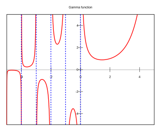
In mathematics, the gamma function is one commonly used extension of the factorial function to complex numbers. The gamma function is defined for all complex numbers except the non-positive integers. For every positive integer n,

In mathematical physics, the Dirac delta distribution, also known as the unit impulse, is a generalized function or distribution over the real numbers, whose value is zero everywhere except at zero, and whose integral over the entire real line is equal to one.

In probability theory, a probability density function (PDF), or density of an absolutely continuous random variable, is a function whose value at any given sample in the sample space can be interpreted as providing a relative likelihood that the value of the random variable would be equal to that sample. Probability density is the probability per unit length, in other words, while the absolute likelihood for a continuous random variable to take on any particular value is 0, the value of the PDF at two different samples can be used to infer, in any particular draw of the random variable, how much more likely it is that the random variable would be close to one sample compared to the other sample.

In physics and mathematics, the Fourier transform (FT) is a transform that converts a function into a form that describes the frequencies present in the original function. The output of the transform is a complex-valued function of frequency. The term Fourier transform refers to both this complex-valued function and the mathematical operation. When a distinction needs to be made the Fourier transform is sometimes called the frequency domain representation of the original function. The Fourier transform is analogous to decomposing the sound of a musical chord into terms of the intensity of its constituent pitches.
A Fourier series is an expansion of a periodic function into a sum of trigonometric functions. The Fourier series is an example of a trigonometric series, but not all trigonometric series are Fourier series. By expressing a function as a sum of sines and cosines, many problems involving the function become easier to analyze because trigonometric functions are well understood. For example, Fourier series were first used by Joseph Fourier to find solutions to the heat equation. This application is possible because the derivatives of trigonometric functions fall into simple patterns. Fourier series cannot be used to approximate arbitrary functions, because most functions have infinitely many terms in their Fourier series, and the series do not always converge. Well-behaved functions, for example smooth functions, have Fourier series that converge to the original function. The coefficients of the Fourier series are determined by integrals of the function multiplied by trigonometric functions, described in Common forms of the Fourier series below.

In complex analysis, the residue theorem, sometimes called Cauchy's residue theorem, is a powerful tool to evaluate line integrals of analytic functions over closed curves; it can often be used to compute real integrals and infinite series as well. It generalizes the Cauchy integral theorem and Cauchy's integral formula. From a geometrical perspective, it can be seen as a special case of the generalized Stokes' theorem.
In complex analysis, a branch of mathematics, analytic continuation is a technique to extend the domain of definition of a given analytic function. Analytic continuation often succeeds in defining further values of a function, for example in a new region where the infinite series representation which initially defined the function becomes divergent.

The Heaviside step function, or the unit step function, usually denoted by H or θ, is a step function named after Oliver Heaviside, the value of which is zero for negative arguments and one for positive arguments. It is an example of the general class of step functions, all of which can be represented as linear combinations of translations of this one.
In algebra, a valuation is a function on a field that provides a measure of the size or multiplicity of elements of the field. It generalizes to commutative algebra the notion of size inherent in consideration of the degree of a pole or multiplicity of a zero in complex analysis, the degree of divisibility of a number by a prime number in number theory, and the geometrical concept of contact between two algebraic or analytic varieties in algebraic geometry. A field with a valuation on it is called a valued field.
In mathematics, more specifically in harmonic analysis, Walsh functions form a complete orthogonal set of functions that can be used to represent any discrete function—just like trigonometric functions can be used to represent any continuous function in Fourier analysis. They can thus be viewed as a discrete, digital counterpart of the continuous, analog system of trigonometric functions on the unit interval. But unlike the sine and cosine functions, which are continuous, Walsh functions are piecewise constant. They take the values −1 and +1 only, on sub-intervals defined by dyadic fractions.
In mathematics, the Poisson summation formula is an equation that relates the Fourier series coefficients of the periodic summation of a function to values of the function's continuous Fourier transform. Consequently, the periodic summation of a function is completely defined by discrete samples of the original function's Fourier transform. And conversely, the periodic summation of a function's Fourier transform is completely defined by discrete samples of the original function. The Poisson summation formula was discovered by Siméon Denis Poisson and is sometimes called Poisson resummation.
In mathematics and signal processing, the Hilbert transform is a specific singular integral that takes a function, u(t) of a real variable and produces another function of a real variable H(u)(t). The Hilbert transform is given by the Cauchy principal value of the convolution with the function (see § Definition). The Hilbert transform has a particularly simple representation in the frequency domain: It imparts a phase shift of ±90° (π⁄2 radians) to every frequency component of a function, the sign of the shift depending on the sign of the frequency (see § Relationship with the Fourier transform). The Hilbert transform is important in signal processing, where it is a component of the analytic representation of a real-valued signal u(t). The Hilbert transform was first introduced by David Hilbert in this setting, to solve a special case of the Riemann–Hilbert problem for analytic functions.
In mathematical analysis, asymptotic analysis, also known as asymptotics, is a method of describing limiting behavior.
In mathematics, the discrete-time Fourier transform (DTFT), also called the finite Fourier transform, is a form of Fourier analysis that is applicable to a sequence of values.
In mathematics, Borel summation is a summation method for divergent series, introduced by Émile Borel (1899). It is particularly useful for summing divergent asymptotic series, and in some sense gives the best possible sum for such series. There are several variations of this method that are also called Borel summation, and a generalization of it called Mittag-Leffler summation.
In probability theory and directional statistics, a wrapped probability distribution is a continuous probability distribution that describes data points that lie on a unit n-sphere. In one dimension, a wrapped distribution consists of points on the unit circle. If is a random variate in the interval with probability density function (PDF) , then is a circular variable distributed according to the wrapped distribution and is an angular variable in the interval distributed according to the wrapped distribution .
In algebra and number theory, a distribution is a function on a system of finite sets into an abelian group which is analogous to an integral: it is thus the algebraic analogue of a distribution in the sense of generalised function.
In mathematics, the Weil–Brezin map, named after André Weil and Jonathan Brezin, is a unitary transformation that maps a Schwartz function on the real line to a smooth function on the Heisenberg manifold. The Weil–Brezin map gives a geometric interpretation of the Fourier transform, the Plancherel theorem and the Poisson summation formula. The image of Gaussian functions under the Weil–Brezin map are nil-theta functions, which are related to theta functions. The Weil–Brezin map is sometimes referred to as the Zak transform, which is widely applied in the field of physics and signal processing; however, the Weil–Brezin Map is defined via Heisenberg group geometrically, whereas there is no direct geometric or group theoretic interpretation from the Zak transform.


