Brownian bridge

Last updated March 22, 2024

A Brownian bridge is a continuous-time stochastic process B(t) whose probability distribution is the conditional probability distribution of a standard Wiener process W(t) (a mathematical model of Brownian motion) subject to the condition (when standardized) that W(T) = 0, so that the process is pinned to the same value at both t = 0 and t = T. More precisely:

The expected value of the bridge at any t in the interval [0,T] is zero, with variance $\textstyle {\frac {t(T-t)}{T}}$ , implying that the most uncertainty is in the middle of the bridge, with zero uncertainty at the nodes. The covariance of B(s) and B(t) is $\min(s,t)-{\frac {s\,t}{T}}$ , or s(T − t)/T if s < t. The increments in a Brownian bridge are not independent.

Relation to other stochastic processes

If W(t) is a standard Wiener process (i.e., for t ≥ 0, W(t) is normally distributed with expected value 0 and variance t, and the increments are stationary and independent), then

B(t)=W(t)-{\frac {t}{T}}W(T)\,

is a Brownian bridge for t ∈ [0, T]. It is independent of W(T)^[1]

Conversely, if B(t) is a Brownian bridge and Z is a standard normal random variable independent of B, then the process

W(t)=B(t)+tZ\,

is a Wiener process for t ∈ [0, 1]. More generally, a Wiener process W(t) for t ∈ [0, T] can be decomposed into

W(t)={\sqrt {T}}B\left({\frac {t}{T}}\right)+{\frac {t}{\sqrt {T}}}Z.

Another representation of the Brownian bridge based on the Brownian motion is, for t ∈ [0, T]

B(t)={\frac {T-t}{\sqrt {T}}}W\left({\frac {t}{T-t}}\right).

Conversely, for t ∈ [0, ∞]

W(t)={\frac {T+t}{T}}B\left({\frac {Tt}{T+t}}\right).

The Brownian bridge may also be represented as a Fourier series with stochastic coefficients, as

B_{t}=\sum _{k=1}^{\infty }Z_{k}{\frac {{\sqrt {2T}}\sin(k\pi t/T)}{k\pi }}

where $Z_{1},Z_{2},\ldots$ are independent identically distributed standard normal random variables (see the Karhunen–Loève theorem).

A Brownian bridge is the result of Donsker's theorem in the area of empirical processes. It is also used in the Kolmogorov–Smirnov test in the area of statistical inference.

Intuitive remarks

A standard Wiener process satisfies W(0) = 0 and is therefore "tied down" to the origin, but other points are not restricted. In a Brownian bridge process on the other hand, not only is B(0) = 0 but we also require that B(T) = 0, that is the process is "tied down" at t = T as well. Just as a literal bridge is supported by pylons at both ends, a Brownian Bridge is required to satisfy conditions at both ends of the interval [0,T]. (In a slight generalization, one sometimes requires B(t₁) = a and B(t₂) = b where t₁, t₂, a and b are known constants.)

Suppose we have generated a number of points W(0), W(1), W(2), W(3), etc. of a Wiener process path by computer simulation. It is now desired to fill in additional points in the interval [0,T], that is to interpolate between the already generated points W(0) and W(T). The solution is to use a Brownian bridge that is required to go through the values W(0) and W(T).

General case

For the general case when B(t₁) = a and B(t₂) = b, the distribution of B at time t ∈ (t₁, t₂) is normal, with mean

a+{\frac {t-t_{1}}{t_{2}-t_{1}}}(b-a)

and variance

{\frac {(t_{2}-t)(t-t_{1})}{t_{2}-t_{1}}},

and the covariance between B(s) and B(t), with s < t is

{\frac {(t_{2}-t)(s-t_{1})}{t_{2}-t_{1}}}.

Related Research Articles

Brownian motion is the random motion of particles suspended in a medium.

In statistics, a normal distribution or Gaussian distribution is a type of continuous probability distribution for a real-valued random variable. The general form of its probability density function is

In mathematics, the Wiener process is a real-valued continuous-time stochastic process named in honor of American mathematician Norbert Wiener for his investigations on the mathematical properties of the one-dimensional Brownian motion. It is often also called Brownian motion due to its historical connection with the physical process of the same name originally observed by Scottish botanist Robert Brown. It is one of the best known Lévy processes and occurs frequently in pure and applied mathematics, economics, quantitative finance, evolutionary biology, and physics.

<span class="mw-page-title-main">Geometric Brownian motion</span> Continuous stochastic process

A geometric Brownian motion (GBM) (also known as exponential Brownian motion) is a continuous-time stochastic process in which the logarithm of the randomly varying quantity follows a Brownian motion (also called a Wiener process) with drift. It is an important example of stochastic processes satisfying a stochastic differential equation (SDE); in particular, it is used in mathematical finance to model stock prices in the Black–Scholes model.

In statistics, the Pearson correlation coefficient (PCC) is a correlation coefficient that measures linear correlation between two sets of data. It is the ratio between the covariance of two variables and the product of their standard deviations; thus, it is essentially a normalized measurement of the covariance, such that the result always has a value between −1 and 1. As with covariance itself, the measure can only reflect a linear correlation of variables, and ignores many other types of relationships or correlations. As a simple example, one would expect the age and height of a sample of teenagers from a high school to have a Pearson correlation coefficient significantly greater than 0, but less than 1.

In mathematics, a random walk, sometimes known as a drunkard's walk, is a random process that describes a path that consists of a succession of random steps on some mathematical space.

In statistics, propagation of uncertainty is the effect of variables' uncertainties on the uncertainty of a function based on them. When the variables are the values of experimental measurements they have uncertainties due to measurement limitations which propagate due to the combination of variables in the function.

In the theory of stochastic processes, the Karhunen–Loève theorem, also known as the Kosambi–Karhunen–Loève theorem states that a stochastic process can be represented as an infinite linear combination of orthogonal functions, analogous to a Fourier series representation of a function on a bounded interval. The transformation is also known as Hotelling transform and eigenvector transform, and is closely related to principal component analysis (PCA) technique widely used in image processing and in data analysis in many fields.

In probability theory, a Lévy process, named after the French mathematician Paul Lévy, is a stochastic process with independent, stationary increments: it represents the motion of a point whose successive displacements are random, in which displacements in pairwise disjoint time intervals are independent, and displacements in different time intervals of the same length have identical probability distributions. A Lévy process may thus be viewed as the continuous-time analog of a random walk.

In probability theory and statistics, the Lévy distribution, named after Paul Lévy, is a continuous probability distribution for a non-negative random variable. In spectroscopy, this distribution, with frequency as the dependent variable, is known as a van der Waals profile. It is a special case of the inverse-gamma distribution. It is a stable distribution.

<span class="mw-page-title-main">Itô calculus</span> Calculus of stochastic differential equations

Itô calculus, named after Kiyosi Itô, extends the methods of calculus to stochastic processes such as Brownian motion. It has important applications in mathematical finance and stochastic differential equations.

In probability theory, fractional Brownian motion (fBm), also called a fractal Brownian motion, is a generalization of Brownian motion. Unlike classical Brownian motion, the increments of fBm need not be independent. fBm is a continuous-time Gaussian process $on, that starts at zero, has expectation zero for all in, and has the following covariance function:$

<span class="mw-page-title-main">Ornstein–Uhlenbeck process</span> Stochastic process modeling random walk with friction

In mathematics, the Ornstein–Uhlenbeck process is a stochastic process with applications in financial mathematics and the physical sciences. Its original application in physics was as a model for the velocity of a massive Brownian particle under the influence of friction. It is named after Leonard Ornstein and George Eugene Uhlenbeck.

In probability theory, Donsker's theorem, named after Monroe D. Donsker, is a functional extension of the central limit theorem for empirical distribution functions. Specifically, the theorem states that an appropriately centered and scaled version of the empirical distribution function converges to a Gaussian process.

In statistics, stochastic volatility models are those in which the variance of a stochastic process is itself randomly distributed. They are used in the field of mathematical finance to evaluate derivative securities, such as options. The name derives from the models' treatment of the underlying security's volatility as a random process, governed by state variables such as the price level of the underlying security, the tendency of volatility to revert to some long-run mean value, and the variance of the volatility process itself, among others.

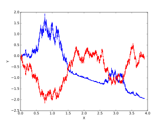
<span class="mw-page-title-main">Brownian excursion</span> Stochastic process

In probability theory a Brownian excursion process is a stochastic process that is closely related to a Wiener process. Realisations of Brownian excursion processes are essentially just realizations of a Wiener process selected to satisfy certain conditions. In particular, a Brownian excursion process is a Wiener process conditioned to be positive and to take the value 0 at time 1. Alternatively, it is a Brownian bridge process conditioned to be positive. BEPs are important because, among other reasons, they naturally arise as the limit process of a number of conditional functional central limit theorems.

In statistics and in probability theory, distance correlation or distance covariance is a measure of dependence between two paired random vectors of arbitrary, not necessarily equal, dimension. The population distance correlation coefficient is zero if and only if the random vectors are independent. Thus, distance correlation measures both linear and nonlinear association between two random variables or random vectors. This is in contrast to Pearson's correlation, which can only detect linear association between two random variables.

In probability theory, reflected Brownian motion is a Wiener process in a space with reflecting boundaries. In the physical literature, this process describes diffusion in a confined space and it is often called confined Brownian motion. For example it can describe the motion of hard spheres in water confined between two walls.

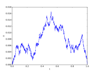
In the mathematical theory of probability, Brownian meander $is a continuous non-homogeneous Markov process defined as follows:$

In physics and mathematics, the Klein–Kramers equation or sometimes referred as Kramers–Chandrasekhar equation is a partial differential equation that describes the probability density function $f$ of a Brownian particle in phase space $(r, p)$ . It is a special case of the Fokker–Planck equation.

References

↑ Aspects of Brownian motion, Springer, 2008, R. Mansuy, M. Yor page 2

Glasserman, Paul (2004). Monte Carlo Methods in Financial Engineering. New York: Springer-Verlag. ISBN 0-387-00451-3.
Revuz, Daniel; Yor, Marc (1999). Continuous Martingales and Brownian Motion (2nd ed.). New York: Springer-Verlag. ISBN 3-540-57622-3.

This page is based on this Wikipedia article
Text is available under the CC BY-SA 4.0 license; additional terms may apply.
Images, videos and audio are available under their respective licenses.

[1] Aspects of Brownian motion, Springer, 2008, R. Mansuy, M. Yor page 2

[1]

v t e Stochastic processes
Discrete time	Bernoulli process Branching process Chinese restaurant process Galton–Watson process Independent and identically distributed random variables Markov chain Moran process Random walk Loop-erased Self-avoiding Biased Maximal entropy
Continuous time	Additive process Bessel process Birth–death process pure birth Brownian motion Bridge Excursion Fractional Geometric Meander Cauchy process Contact process Continuous-time random walk Cox process Diffusion process Dyson Brownian motion Empirical process Feller process Fleming–Viot process Gamma process Geometric process Hawkes process Hunt process Interacting particle systems Itô diffusion Itô process Jump diffusion Jump process Lévy process Local time Markov additive process McKean–Vlasov process Ornstein–Uhlenbeck process Poisson process Compound Non-homogeneous Schramm–Loewner evolution Semimartingale Sigma-martingale Stable process Superprocess Telegraph process Variance gamma process Wiener process Wiener sausage
Both	Branching process Galves–Löcherbach model Gaussian process Hidden Markov model (HMM) Markov process Martingale Differences Local Sub- Super- Random dynamical system Regenerative process Renewal process Stochastic chains with memory of variable length White noise
Fields and other	Dirichlet process Gaussian random field Gibbs measure Hopfield model Ising model Potts model Boolean network Markov random field Percolation Pitman–Yor process Point process Cox Poisson Random field Random graph
Time series models	Autoregressive conditional heteroskedasticity (ARCH) model Autoregressive integrated moving average (ARIMA) model Autoregressive (AR) model Autoregressive–moving-average (ARMA) model Generalized autoregressive conditional heteroskedasticity (GARCH) model Moving-average (MA) model
Financial models	Binomial options pricing model Black–Derman–Toy Black–Karasinski Black–Scholes Chan–Karolyi–Longstaff–Sanders (CKLS) Chen Constant elasticity of variance (CEV) Cox–Ingersoll–Ross (CIR) Garman–Kohlhagen Heath–Jarrow–Morton (HJM) Heston Ho–Lee Hull–White Korn-Kreer-Lenssen LIBOR market Rendleman–Bartter SABR volatility Vašíček Wilkie
Actuarial models	Bühlmann Cramér–Lundberg Risk process Sparre–Anderson
Queueing models	Bulk Fluid Generalized queueing network M/G/1 M/M/1 M/M/c
Properties	Càdlàg paths Continuous Continuous paths Ergodic Exchangeable Feller-continuous Gauss–Markov Markov Mixing Piecewise-deterministic Predictable Progressively measurable Self-similar Stationary Time-reversible
Limit theorems	Central limit theorem Donsker's theorem Doob's martingale convergence theorems Ergodic theorem Fisher–Tippett–Gnedenko theorem Large deviation principle Law of large numbers (weak/strong) Law of the iterated logarithm Maximal ergodic theorem Sanov's theorem Zero–one laws (Blumenthal, Borel–Cantelli, Engelbert–Schmidt, Hewitt–Savage, Kolmogorov, Lévy)
Inequalities	Burkholder–Davis–Gundy Doob's martingale Doob's upcrossing Kunita–Watanabe Marcinkiewicz–Zygmund
Tools	Cameron–Martin formula Convergence of random variables Doléans-Dade exponential Doob decomposition theorem Doob–Meyer decomposition theorem Doob's optional stopping theorem Dynkin's formula Feynman–Kac formula Filtration Girsanov theorem Infinitesimal generator Itô integral Itô's lemma Karhunen–Loève theorem Kolmogorov continuity theorem Kolmogorov extension theorem Lévy–Prokhorov metric Malliavin calculus Martingale representation theorem Optional stopping theorem Prokhorov's theorem Quadratic variation Reflection principle Skorokhod integral Skorokhod's representation theorem Skorokhod space Snell envelope Stochastic differential equation Tanaka Stopping time Stratonovich integral Uniform integrability Usual hypotheses Wiener space Classical Abstract
Disciplines	Actuarial mathematics Control theory Econometrics Ergodic theory Extreme value theory (EVT) Large deviations theory Mathematical finance Mathematical statistics Probability theory Queueing theory Renewal theory Ruin theory Signal processing Statistics Stochastic analysis Time series analysis Machine learning
List of topics Category