SABR volatility model

Last updated February 20, 2024

In mathematical finance, the SABR model is a stochastic volatility model, which attempts to capture the volatility smile in derivatives markets. The name stands for "stochastic alpha, beta, rho", referring to the parameters of the model. The SABR model is widely used by practitioners in the financial industry, especially in the interest rate derivative markets. It was developed by Patrick S. Hagan, Deep Kumar, Andrew Lesniewski, and Diana Woodward.^[1]

Dynamics

The SABR model describes a single forward $F$ , such as a LIBOR forward rate, a forward swap rate, or a forward stock price. This is one of the standards in market used by market participants to quote volatilities. The volatility of the forward $F$ is described by a parameter $\sigma$ . SABR is a dynamic model in which both $F$ and $\sigma$ are represented by stochastic state variables whose time evolution is given by the following system of stochastic differential equations:

dF_{t}=\sigma _{t}\left(F_{t}\right)^{\beta }\,dW_{t},

d\sigma _{t}=\alpha \sigma _{t}^{}\,dZ_{t},

with the prescribed time zero (currently observed) values $F_{0}$ and $\sigma _{0}$ . Here, $W_{t}$ and $Z_{t}$ are two correlated Wiener processes with correlation coefficient $-1<\rho <1$ :

dW_{t}\,dZ_{t}=\rho \,dt

The constant parameters $\beta ,\;\alpha$ satisfy the conditions $0\leq \beta \leq 1,\;\alpha \geq 0$ . $\alpha$ is a volatility-like parameter for the volatility. $\rho$ is the instantaneous correlation between the underlying and its volatility. The initial volatility $\sigma _{0}$ controls the height of the ATM implied volatility level. Both the correlation $\rho$ and $\beta$ controls the slope of the implied skew. The volatiltiy of volatility $\alpha$ controls its curvature.

The above dynamics is a stochastic version of the CEV model with the skewness parameter $\beta$ : in fact, it reduces to the CEV model if $\alpha =0$ The parameter $\alpha$ is often referred to as the volvol, and its meaning is that of the lognormal volatility of the volatility parameter $\sigma$ .

Asymptotic solution

We consider a European option (say, a call) on the forward $F$ struck at $K$ , which expires $T$ years from now. The value of this option is equal to the suitably discounted expected value of the payoff $\max(F_{T}-K,\;0)$ under the probability distribution of the process $F_{t}$ .

Except for the special cases of $\beta =0$ and $\beta =1$ , no closed form expression for this probability distribution is known. The general case can be solved approximately by means of an asymptotic expansion in the parameter $\varepsilon =T\alpha ^{2}$ . Under typical market conditions, this parameter is small and the approximate solution is actually quite accurate. Also significantly, this solution has a rather simple functional form, is very easy to implement in computer code, and lends itself well to risk management of large portfolios of options in real time.

It is convenient to express the solution in terms of the implied volatility $\sigma _{\textrm {impl}}$ of the option. Namely, we force the SABR model price of the option into the form of the Black model valuation formula. Then the implied volatility, which is the value of the lognormal volatility parameter in Black's model that forces it to match the SABR price, is approximately given by:

\sigma _{\text{impl}}=\alpha \;{\frac {\log(F_{0}/K)}{D(\zeta )}}\;\left\{1+\left[{\frac {2\gamma _{2}-\gamma _{1}^{2}+1/\left(F_{\text{mid}}\right)^{2}}{24}}\;\left({\frac {\sigma _{0}C(F_{\text{mid}})}{\alpha }}\right)^{2}+{\frac {\rho \gamma _{1}}{4}}\;{\frac {\sigma _{0}C(F_{\text{mid}})}{\alpha }}+{\frac {2-3\rho ^{2}}{24}}\right]\varepsilon \right\},

where, for clarity, we have set $C\left(F\right)=F^{\beta }$ . The value $F_{\text{mid}}$ denotes a conveniently chosen midpoint between $F_{0}$ and $K$ (such as the geometric average ${\sqrt {F_{0}K}}$ or the arithmetic average $\left(F_{0}+K\right)/2$ ). We have also set

\zeta ={\frac {\alpha }{\sigma _{0}}}\;\int _{K}^{F_{0}}{\frac {dx}{C(x)}}={\frac {\alpha }{\sigma _{0}(1-\beta )}}\;\left(F_{0}{}^{1-\beta }-K^{1-\beta }\right),

and

\gamma _{1}={\frac {C'(F_{\text{mid}})}{C(F_{\text{mid}})}}={\frac {\beta }{F_{\text{mid}}}}\;,

\gamma _{2}={\frac {C''(F_{\text{mid}})}{C(F_{\text{mid}})}}=-{\frac {\beta (1-\beta )}{\left(F_{\text{mid}}\right)^{2}}}\;,

The function $D\left(\zeta \right)$ entering the formula above is given by

D(\zeta )=\log \left({\frac {{\sqrt {1-2\rho \zeta +\zeta ^{2}}}+\zeta -\rho }{1-\rho }}\right).

Alternatively, one can express the SABR price in terms of the Bachelier's model. Then the implied normal volatility can be asymptotically computed by means of the following expression:

\sigma _{\text{impl}}^{\text{n}}=\alpha \;{\frac {F_{0}-K}{D(\zeta )}}\;\left\{1+\left[{\frac {2\gamma _{2}-\gamma _{1}^{2}}{24}}\;\left({\frac {\sigma _{0}C(F_{\text{mid}})}{\alpha }}\right)^{2}+{\frac {\rho \gamma _{1}}{4}}\;{\frac {\sigma _{0}C(F_{\text{mid}})}{\alpha }}+{\frac {2-3\rho ^{2}}{24}}\right]\varepsilon \right\}.

It is worth noting that the normal SABR implied volatility is generally somewhat more accurate than the lognormal implied volatility.

The approximation accuracy and the degree of arbitrage can be further improved if the equivalent volatility under the CEV model with the same $\beta$ is used for pricing options.^[2]

SABR for the negative rates

A SABR model extension for negative interest rates that has gained popularity in recent years is the shifted SABR model, where the shifted forward rate is assumed to follow a SABR process

dF_{t}=\sigma _{t}(F_{t}+s)^{\beta }\,dW_{t},

d\sigma _{t}=\alpha \sigma _{t}\,dZ_{t},

for some positive shift $s$ . Since shifts are included in a market quotes, and there is an intuitive soft boundary for how negative rates can become, shifted SABR has become market best practice to accommodate negative rates.

The SABR model can also be modified to cover negative interest rates by:

dF_{t}=\sigma _{t}|F_{t}|^{\beta }\,dW_{t},

d\sigma _{t}=\alpha \sigma _{t}\,dZ_{t},

for $0\leq \beta \leq 1/2$ and a free boundary condition for $F=0$ . Its exact solution for the zero correlation as well as an efficient approximation for a general case are available.^[3] An obvious drawback of this approach is the a priori assumption of potential highly negative interest rates via the free boundary.

Arbitrage problem in the implied volatility formula

Although the asymptotic solution is very easy to implement, the density implied by the approximation is not always arbitrage-free, especially not for very low strikes (it becomes negative or the density does not integrate to one).

One possibility to "fix" the formula is use the stochastic collocation method and to project the corresponding implied, ill-posed, model on a polynomial of an arbitrage-free variables, e.g. normal. This will guarantee equality in probability at the collocation points while the generated density is arbitrage-free.^[4] Using the projection method analytic European option prices are available and the implied volatilities stay very close to those initially obtained by the asymptotic formula.

Another possibility is to rely on a fast and robust PDE solver on an equivalent expansion of the forward PDE, that preserves numerically the zero-th and first moment, thus guaranteeing the absence of arbitrage.^[5]

Extensions

The SABR model can be extended by assuming its parameters to be time-dependent. This however complicates the calibration procedure. An advanced calibration method of the time-dependent SABR model is based on so-called "effective parameters".^[6]

Alternatively, Guerrero and Orlando ^[7] show that a time-dependent local stochastic volatility (SLV) model can be reduced to a system of autonomous PDEs that can be solved using the heat kernel, by means of the Wei-Norman factorization method and Lie algebraic techniques. Explicit solutions obtained by said techniques are comparable to traditional Monte Carlo simulations allowing for shorter time in numerical computations.

Simulation

As the stochastic volatility process follows a geometric Brownian motion, its exact simulation is straightforward. However, the simulation of the forward asset process is not a trivial task. Taylor-based simulation schemes are typically considered, like Euler–Maruyama or Milstein. Recently, novel methods have been proposed for the almost exact Monte Carlo simulation of the SABR model.^[8] Extensive studies for SABR model have recently been considered.^[9] For the normal SABR model ( $\beta =0$ with no boundary condition at $F=0$ ), a closed-form simulation method is known.^[10]

Related Research Articles

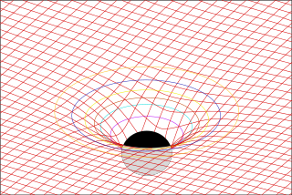
In the mathematical field of differential geometry, the Riemann curvature tensor or Riemann–Christoffel tensor is the most common way used to express the curvature of Riemannian manifolds. It assigns a tensor to each point of a Riemannian manifold. It is a local invariant of Riemannian metrics which measures the failure of the second covariant derivatives to commute. A Riemannian manifold has zero curvature if and only if it is flat, i.e. locally isometric to the Euclidean space. The curvature tensor can also be defined for any pseudo-Riemannian manifold, or indeed any manifold equipped with an affine connection.

In econometrics, the autoregressive conditional heteroskedasticity (ARCH) model is a statistical model for time series data that describes the variance of the current error term or innovation as a function of the actual sizes of the previous time periods' error terms; often the variance is related to the squares of the previous innovations. The ARCH model is appropriate when the error variance in a time series follows an autoregressive (AR) model; if an autoregressive moving average (ARMA) model is assumed for the error variance, the model is a generalized autoregressive conditional heteroskedasticity (GARCH) model.

In financial mathematics, the Hull–White model is a model of future interest rates. In its most generic formulation, it belongs to the class of no-arbitrage models that are able to fit today's term structure of interest rates. It is relatively straightforward to translate the mathematical description of the evolution of future interest rates onto a tree or lattice and so interest rate derivatives such as bermudan swaptions can be valued in the model.

In physics, precisely in the study of the theory of general relativity and many alternatives to it, the post-Newtonian formalism is a calculational tool that expresses Einstein's (nonlinear) equations of gravity in terms of the lowest-order deviations from Newton's law of universal gravitation. This allows approximations to Einstein's equations to be made in the case of weak fields. Higher-order terms can be added to increase accuracy, but for strong fields, it may be preferable to solve the complete equations numerically. Some of these post-Newtonian approximations are expansions in a small parameter, which is the ratio of the velocity of the matter forming the gravitational field to the speed of light, which in this case is better called the speed of gravity. In the limit, when the fundamental speed of gravity becomes infinite, the post-Newtonian expansion reduces to Newton's law of gravity.

In relativistic physics, the electromagnetic stress–energy tensor is the contribution to the stress–energy tensor due to the electromagnetic field. The stress–energy tensor describes the flow of energy and momentum in spacetime. The electromagnetic stress–energy tensor contains the negative of the classical Maxwell stress tensor that governs the electromagnetic interactions.

The covariant formulation of classical electromagnetism refers to ways of writing the laws of classical electromagnetism in a form that is manifestly invariant under Lorentz transformations, in the formalism of special relativity using rectilinear inertial coordinate systems. These expressions both make it simple to prove that the laws of classical electromagnetism take the same form in any inertial coordinate system, and also provide a way to translate the fields and forces from one frame to another. However, this is not as general as Maxwell's equations in curved spacetime or non-rectilinear coordinate systems.

In physics, Maxwell's equations in curved spacetime govern the dynamics of the electromagnetic field in curved spacetime or where one uses an arbitrary coordinate system. These equations can be viewed as a generalization of the vacuum Maxwell's equations which are normally formulated in the local coordinates of flat spacetime. But because general relativity dictates that the presence of electromagnetic fields induce curvature in spacetime, Maxwell's equations in flat spacetime should be viewed as a convenient approximation.

In the theory of general relativity, a stress–energy–momentum pseudotensor, such as the Landau–Lifshitz pseudotensor, is an extension of the non-gravitational stress–energy tensor that incorporates the energy–momentum of gravity. It allows the energy–momentum of a system of gravitating matter to be defined. In particular it allows the total of matter plus the gravitating energy–momentum to form a conserved current within the framework of general relativity, so that the total energy–momentum crossing the hypersurface of any compact space–time hypervolume vanishes.

In statistics, stochastic volatility models are those in which the variance of a stochastic process is itself randomly distributed. They are used in the field of mathematical finance to evaluate derivative securities, such as options. The name derives from the models' treatment of the underlying security's volatility as a random process, governed by state variables such as the price level of the underlying security, the tendency of volatility to revert to some long-run mean value, and the variance of the volatility process itself, among others.

The Newman–Penrose (NP) formalism is a set of notation developed by Ezra T. Newman and Roger Penrose for general relativity (GR). Their notation is an effort to treat general relativity in terms of spinor notation, which introduces complex forms of the usual variables used in GR. The NP formalism is itself a special case of the tetrad formalism, where the tensors of the theory are projected onto a complete vector basis at each point in spacetime. Usually this vector basis is chosen to reflect some symmetry of the spacetime, leading to simplified expressions for physical observables. In the case of the NP formalism, the vector basis chosen is a null tetrad: a set of four null vectors—two real, and a complex-conjugate pair. The two real members often asymptotically point radially inward and radially outward, and the formalism is well adapted to treatment of the propagation of radiation in curved spacetime. The Weyl scalars, derived from the Weyl tensor, are often used. In particular, it can be shown that one of these scalars— $in the appropriate frame—encodes the outgoing gravitational radiation of an asymptotically flat system.$

Bayesian linear regression is a type of conditional modeling in which the mean of one variable is described by a linear combination of other variables, with the goal of obtaining the posterior probability of the regression coefficients and ultimately allowing the out-of-sample prediction of the regressandconditional on observed values of the regressors. The simplest and most widely used version of this model is the normal linear model, in which $given is distributed Gaussian. In this model, and under a particular choice of prior probabilities for the parameters—so-called conjugate priors—the posterior can be found analytically. With more arbitrarily chosen priors, the posteriors generally have to be approximated.$

<span class="mw-page-title-main">Cox–Ingersoll–Ross model</span> Stochastic model for the evolution of financial interest rates

In mathematical finance, the Cox–Ingersoll–Ross (CIR) model describes the evolution of interest rates. It is a type of "one factor model" as it describes interest rate movements as driven by only one source of market risk. The model can be used in the valuation of interest rate derivatives. It was introduced in 1985 by John C. Cox, Jonathan E. Ingersoll and Stephen A. Ross as an extension of the Vasicek model.

A ratio distribution is a probability distribution constructed as the distribution of the ratio of random variables having two other known distributions. Given two random variables X and Y, the distribution of the random variable Z that is formed as the ratio Z = X/Y is a ratio distribution.

Fluid films, such as soap films, are commonly encountered in everyday experience. A soap film can be formed by dipping a closed contour wire into a soapy solution as in the figure on the right. Alternatively, a catenoid can be formed by dipping two rings in the soapy solution and subsequently separating them while maintaining the coaxial configuration.

In theoretical physics, Lovelock's theory of gravity (often referred to as Lovelock gravity) is a generalization of Einstein's theory of general relativity introduced by David Lovelock in 1971. It is the most general metric theory of gravity yielding conserved second order equations of motion in an arbitrary number of spacetime dimensions D. In this sense, Lovelock's theory is the natural generalization of Einstein's general relativity to higher dimensions. In three and four dimensions (D = 3, 4), Lovelock's theory coincides with Einstein's theory, but in higher dimensions the theories are different. In fact, for D > 4 Einstein gravity can be thought of as a particular case of Lovelock gravity since the Einstein–Hilbert action is one of several terms that constitute the Lovelock action.

In mathematics, Ricci calculus constitutes the rules of index notation and manipulation for tensors and tensor fields on a differentiable manifold, with or without a metric tensor or connection. It is also the modern name for what used to be called the absolute differential calculus, developed by Gregorio Ricci-Curbastro in 1887–1896, and subsequently popularized in a paper written with his pupil Tullio Levi-Civita in 1900. Jan Arnoldus Schouten developed the modern notation and formalism for this mathematical framework, and made contributions to the theory, during its applications to general relativity and differential geometry in the early twentieth century.

In queueing theory, a discipline within the mathematical theory of probability, a heavy traffic approximation is the matching of a queueing model with a diffusion process under some limiting conditions on the model's parameters. The first such result was published by John Kingman who showed that when the utilisation parameter of an M/M/1 queue is near 1 a scaled version of the queue length process can be accurately approximated by a reflected Brownian motion.

Stochastic portfolio theory (SPT) is a mathematical theory for analyzing stock market structure and portfolio behavior introduced by E. Robert Fernholz in 2002. It is descriptive as opposed to normative, and is consistent with the observed behavior of actual markets. Normative assumptions, which serve as a basis for earlier theories like modern portfolio theory (MPT) and the capital asset pricing model (CAPM), are absent from SPT.

The generalized functional linear model (GFLM) is an extension of the generalized linear model (GLM) that allows one to regress univariate responses of various types on functional predictors, which are mostly random trajectories generated by a square-integrable stochastic processes. Similarly to GLM, a link function relates the expected value of the response variable to a linear predictor, which in case of GFLM is obtained by forming the scalar product of the random predictor function $with a smooth parameter function . Functional Linear Regression, Functional Poisson Regression and Functional Binomial Regression, with the important Functional Logistic Regression included, are special cases of GFLM. Applications of GFLM include classification and discrimination of stochastic processes and functional data.$

In machine learning, diffusion models, also known as diffusion probabilistic models or score-based generative models, are a class of latent variable generative models. A diffusion model consists of three major components: the forward process, the reverse process, and the sampling procedure. The goal of diffusion models is to learn a diffusion process that generates the probability distribution of a given dataset. They learn the latent structure of a dataset by modeling the way in which data points diffuse through their latent space.

References

↑ Hagan, Patrick S.; Kumar, Deep; Kesniewski, Andrew S.; Woodward, Diana E. (January 2002). "Managing Smile Risk" (PDF). Wilmott . Vol. 1. pp. 84–108. Archived (PDF) from the original on 2022-04-30. Retrieved 2022-04-30.
↑ Choi, Jaehyuk; Wu, Lixin (July 2021). "The equivalent constant-elasticity-of-variance (CEV) volatility of the stochastic-alpha-beta-rho (SABR) model". Journal of Economic Dynamics and Control . 128: 104143. arXiv: 1911.13123 . doi:10.1016/j.jedc.2021.104143. S2CID 235239799. SSRN 3495464 . Retrieved 2022-04-30.
↑ Antonov, Alexandre; Konikov, Michael; Spector, Michael (2015-01-28). "The Free Boundary SABR: Natural Extension to Negative Rates". SSRN 2557046.
↑ Grzelak, Lech A.; Oosterlee, Cornelis W. (February 2017) [2016-07-04]. "From arbitrage to arbitrage-free implied volatilities". Journal of Computational Finance. 20 (3): 31–49. doi:10.21314/JCF.2016.316. ISSN 1755-2850. SSRN 2529684 . Retrieved 2022-04-30.
↑ Le Floc'h, Fabien; Kennedy, Gary (2016-08-15). "Finite difference techniques for arbitrage-free SABR". Journal of Computational Finance. ISSN 1755-2850 . Retrieved 2022-04-30.
↑ Van der Stoep, Anton W.; Grzelak, Lech Aleksander; Oosterlee, Cornelis W. (2015-09-28). "The Time-Dependent FX-SABR Model: Efficient Calibration based on Effective Parameters". International Journal of Theoretical and Applied Finance . 18 (6): 1550042. doi:10.1142/S0219024915500429. SSRN 2503891 . Retrieved 2022-04-30.
↑ Guerrero, Julio; Orlando, Giuseppe (September 2021). "Stochastic local volatility models and the Wei-Norman factorization method". Discrete & Continuous Dynamical Systems - S. 15 (12): 3699–3722. arXiv: 2201.11241 . doi:10.3934/dcdss.2022026. ISSN 1937-1632. S2CID 246295004 . Retrieved 2022-04-30.
↑ Leitao, Álvaro; Grzelak, Lech A.; Oosterlee, Cornelis W. (2017-04-10) [2016-04-13]. "On an efficient multiple time step Monte Carlo simulation of the SABR model". Quantitative Finance. 17 (10): 1549–1565. doi: 10.1080/14697688.2017.1301676 . SSRN 2764908.
↑ Cui, Zhenyu; Kirkby, Justin L.; Nguyen, Duy (2018-04-24). "A General Valuation Framework for SABR and Stochastic Local Volatility Models". SIAM Journal on Financial Mathematics. 9 (2): 520–563. doi:10.1137/16M1106572. S2CID 207074154.
↑ Choi, Jaehyuk; Liu, Chenru; Seo, Byoung Ki (2018-10-31). "Hyperbolic normal stochastic volatility model". Journal of Futures Markets . 39 (2): 186–204. arXiv: 1809.04035 . doi:10.1002/fut.21967. S2CID 158662660. SSRN 3068836 . Retrieved 2022-04-30.

v t e Volatility
Modelling volatility	Implied volatility Volatility smile Volatility clustering Local volatility Stochastic volatility Jump-diffusion models ARCH and GARCH
Trading volatility	Volatility arbitrage Straddle Volatility swap IVX VIX

v t e Stochastic processes
Discrete time	Bernoulli process Branching process Chinese restaurant process Galton–Watson process Independent and identically distributed random variables Markov chain Moran process Random walk Loop-erased Self-avoiding Biased Maximal entropy
Continuous time	Additive process Bessel process Birth–death process pure birth Brownian motion Bridge Excursion Fractional Geometric Meander Cauchy process Contact process Continuous-time random walk Cox process Diffusion process Dyson Brownian motion Empirical process Feller process Fleming–Viot process Gamma process Geometric process Hawkes process Hunt process Interacting particle systems Itô diffusion Itô process Jump diffusion Jump process Lévy process Local time Markov additive process McKean–Vlasov process Ornstein–Uhlenbeck process Poisson process Compound Non-homogeneous Schramm–Loewner evolution Semimartingale Sigma-martingale Stable process Superprocess Telegraph process Variance gamma process Wiener process Wiener sausage
Both	Branching process Galves–Löcherbach model Gaussian process Hidden Markov model (HMM) Markov process Martingale Differences Local Sub- Super- Random dynamical system Regenerative process Renewal process Stochastic chains with memory of variable length White noise
Fields and other	Dirichlet process Gaussian random field Gibbs measure Hopfield model Ising model Potts model Boolean network Markov random field Percolation Pitman–Yor process Point process Cox Poisson Random field Random graph
Time series models	Autoregressive conditional heteroskedasticity (ARCH) model Autoregressive integrated moving average (ARIMA) model Autoregressive (AR) model Autoregressive–moving-average (ARMA) model Generalized autoregressive conditional heteroskedasticity (GARCH) model Moving-average (MA) model
Financial models	Binomial options pricing model Black–Derman–Toy Black–Karasinski Black–Scholes Chan–Karolyi–Longstaff–Sanders (CKLS) Chen Constant elasticity of variance (CEV) Cox–Ingersoll–Ross (CIR) Garman–Kohlhagen Heath–Jarrow–Morton (HJM) Heston Ho–Lee Hull–White Korn-Kreer-Lenssen LIBOR market Rendleman–Bartter SABR volatility Vašíček Wilkie
Actuarial models	Bühlmann Cramér–Lundberg Risk process Sparre–Anderson
Queueing models	Bulk Fluid Generalized queueing network M/G/1 M/M/1 M/M/c
Properties	Càdlàg paths Continuous Continuous paths Ergodic Exchangeable Feller-continuous Gauss–Markov Markov Mixing Piecewise-deterministic Predictable Progressively measurable Self-similar Stationary Time-reversible
Limit theorems	Central limit theorem Donsker's theorem Doob's martingale convergence theorems Ergodic theorem Fisher–Tippett–Gnedenko theorem Large deviation principle Law of large numbers (weak/strong) Law of the iterated logarithm Maximal ergodic theorem Sanov's theorem Zero–one laws (Blumenthal, Borel–Cantelli, Engelbert–Schmidt, Hewitt–Savage, Kolmogorov, Lévy)
Inequalities	Burkholder–Davis–Gundy Doob's martingale Doob's upcrossing Kunita–Watanabe Marcinkiewicz–Zygmund
Tools	Cameron–Martin formula Convergence of random variables Doléans-Dade exponential Doob decomposition theorem Doob–Meyer decomposition theorem Doob's optional stopping theorem Dynkin's formula Feynman–Kac formula Filtration Girsanov theorem Infinitesimal generator Itô integral Itô's lemma Karhunen–Loève theorem Kolmogorov continuity theorem Kolmogorov extension theorem Lévy–Prokhorov metric Malliavin calculus Martingale representation theorem Optional stopping theorem Prokhorov's theorem Quadratic variation Reflection principle Skorokhod integral Skorokhod's representation theorem Skorokhod space Snell envelope Stochastic differential equation Tanaka Stopping time Stratonovich integral Uniform integrability Usual hypotheses Wiener space Classical Abstract
Disciplines	Actuarial mathematics Control theory Econometrics Ergodic theory Extreme value theory (EVT) Large deviations theory Mathematical finance Mathematical statistics Probability theory Queueing theory Renewal theory Ruin theory Signal processing Statistics Stochastic analysis Time series analysis Machine learning
List of topics Category