Dirichlet process

Last updated
Draws from the Dirichlet process
DP
[?]
(
N
(
0
,
1
)
,
a
)
{\displaystyle \operatorname {DP} (N(0,1),\alpha )}
. The four rows use different alpha
a
{\displaystyle \alpha }
(top to bottom: 1, 10, 100 and 1000) and each row contains three repetitions of the same experiment. As seen from the graphs, draws from a Dirichlet process are discrete distributions and they become less concentrated (more spread out) with increasing
a
{\displaystyle \alpha }
. The graphs were generated using the stick-breaking process view of the Dirichlet process. Dirichlet process draws.svg
Draws from the Dirichlet process . The four rows use different alpha (top to bottom: 1, 10, 100 and 1000) and each row contains three repetitions of the same experiment. As seen from the graphs, draws from a Dirichlet process are discrete distributions and they become less concentrated (more spread out) with increasing . The graphs were generated using the stick-breaking process view of the Dirichlet process.

In probability theory, Dirichlet processes (after the distribution associated with Peter Gustav Lejeune Dirichlet) are a family of stochastic processes whose realizations are probability distributions. In other words, a Dirichlet process is a probability distribution whose range is itself a set of probability distributions. It is often used in Bayesian inference to describe the prior knowledge about the distribution of random variables how likely it is that the random variables are distributed according to one or another particular distribution.

Contents

As an example, a bag of 100 real-world dice is a random probability mass function (random pmf)—to sample this random pmf you put your hand in the bag and draw out a die, that is, you draw a pmf. A bag of dice manufactured using a crude process 100 years ago will likely have probabilities that deviate wildly from the uniform pmf, whereas a bag of state-of-the-art dice used by Las Vegas casinos may have barely perceptible imperfections. We can model the randomness of pmfs with the Dirichlet distribution. [1]

The Dirichlet process is specified by a base distribution and a positive real number called the concentration parameter (also known as scaling parameter). The base distribution is the expected value of the process, i.e., the Dirichlet process draws distributions "around" the base distribution the way a normal distribution draws real numbers around its mean. However, even if the base distribution is continuous, the distributions drawn from the Dirichlet process are almost surely discrete. The scaling parameter specifies how strong this discretization is: in the limit of , the realizations are all concentrated at a single value, while in the limit of the realizations become continuous. Between the two extremes the realizations are discrete distributions with less and less concentration as increases.

The Dirichlet process can also be seen as the infinite-dimensional generalization of the Dirichlet distribution. In the same way as the Dirichlet distribution is the conjugate prior for the categorical distribution, the Dirichlet process is the conjugate prior for infinite, nonparametric discrete distributions. A particularly important application of Dirichlet processes is as a prior probability distribution in infinite mixture models.

The Dirichlet process was formally introduced by Thomas S. Ferguson in 1973. [2] It has since been applied in data mining and machine learning, among others for natural language processing, computer vision and bioinformatics.

Introduction

Dirichlet processes are usually used when modelling data that tends to repeat previous values in a so-called "rich get richer" fashion. Specifically, suppose that the generation of values can be simulated by the following algorithm.

Input: (a probability distribution called base distribution), (a positive real number called scaling parameter)
For :

a) With probability draw Failed to parse (SVG (MathML can be enabled via browser plugin): Invalid response ("Math extension cannot connect to Restbase.") from server "http://localhost:6011/en.wikipedia.org/v1/":): {\displaystyle X_n} from .

b) With probability set , where is the number of previous observations of .
(Formally, where denotes the number of elements in the set.)

At the same time, another common model for data is that the observations are assumed to be independent and identically distributed (i.i.d.) according to some (random) distribution . The goal of introducing Dirichlet processes is to be able to describe the procedure outlined above in this i.i.d. model.

The observations in the algorithm are not independent, since we have to consider the previous results when generating the next value. They are, however, exchangeable. This fact can be shown by calculating the joint probability distribution of the observations and noticing that the resulting formula only depends on which values occur among the observations and how many repetitions they each have. Because of this exchangeability, de Finetti's representation theorem applies and it implies that the observations are conditionally independent given a (latent) distribution . This is a random variable itself and has a distribution. This distribution (over distributions) is called a Dirichlet process (). In summary, this means that we get an equivalent procedure to the above algorithm:

  1. Draw a distribution from
  2. Draw observations independently from .

In practice, however, drawing a concrete distribution is impossible, since its specification requires an infinite amount of information. This is a common phenomenon in the context of Bayesian non-parametric statistics where a typical task is to learn distributions on function spaces, which involve effectively infinitely many parameters. The key insight is that in many applications the infinite-dimensional distributions appear only as an intermediary computational device and are not required for either the initial specification of prior beliefs or for the statement of the final inference.

Formal definition

Given a measurable set S, a base probability distribution H and a positive real number , the Dirichlet process is a stochastic process whose sample path (or realization, i.e. an infinite sequence of random variates drawn from the process) is a probability distribution over S, such that the following holds. For any measurable finite partition of S, denoted ,

where denotes the Dirichlet distribution and the notation means that the random variable has the distribution .

Alternative views

There are several equivalent views of the Dirichlet process. Besides the formal definition above, the Dirichlet process can be defined implicitly through de Finetti's theorem as described in the first section; this is often called the Chinese restaurant process. A third alternative is the stick-breaking process, which defines the Dirichlet process constructively by writing a distribution sampled from the process as , where are samples from the base distribution , is an indicator function centered on (zero everywhere except for ) and the are defined by a recursive scheme that repeatedly samples from the beta distribution .

The Chinese restaurant process

Animation of a Chinese restaurant process with scaling parameter . Tables are hidden once the customers of a table can not be displayed anymore; however, every table has infinitely many seats. (Recording of an interactive animation. [3] )

A widely employed metaphor for the Dirichlet process is based on the so-called Chinese restaurant process. The metaphor is as follows:

Imagine a Chinese restaurant in which customers enter. A new customer sits down at a table with a probability proportional to the number of customers already sitting there. Additionally, a customer opens a new table with a probability proportional to the scaling parameter . After infinitely many customers entered, one obtains a probability distribution over infinitely many tables to be chosen. This probability distribution over the tables is a random sample of the probabilities of observations drawn from a Dirichlet process with scaling parameter .

If one associates draws from the base measure with every table, the resulting distribution over the sample space is a random sample of a Dirichlet process. The Chinese restaurant process is related to the Pólya urn sampling scheme which yields samples from finite Dirichlet distributions.

Because customers sit at a table with a probability proportional to the number of customers already sitting at the table, two properties of the DP can be deduced:

  1. The Dirichlet process exhibits a self-reinforcing property: The more often a given value has been sampled in the past, the more likely it is to be sampled again.
  2. Even if is a distribution over an uncountable set, there is a nonzero probability that two samples will have exactly the same value because the probability mass will concentrate on a small number of tables.

The stick-breaking process

A third approach to the Dirichlet process is the so-called stick-breaking process view. Conceptually, this involves repeatedly breaking off and discarding a random fraction (sampled from a Beta distribution) of a "stick" that is initially of length 1. Remember that draws from a Dirichlet process are distributions over a set . As noted previously, the distribution drawn is discrete with probability 1. In the stick-breaking process view, we explicitly use the discreteness and give the probability mass function of this (random) discrete distribution as:

where is the indicator function which evaluates to zero everywhere, except for . Since this distribution is random itself, its mass function is parameterized by two sets of random variables: the locations and the corresponding probabilities . In the following, we present without proof what these random variables are.

The locations are independent and identically distributed according to , the base distribution of the Dirichlet process. The probabilities are given by a procedure resembling the breaking of a unit-length stick (hence the name):

where are independent random variables with the beta distribution . The resemblance to 'stick-breaking' can be seen by considering as the length of a piece of a stick. We start with a unit-length stick and in each step we break off a portion of the remaining stick according to and assign this broken-off piece to . The formula can be understood by noting that after the first k  1 values have their portions assigned, the length of the remainder of the stick is and this piece is broken according to and gets assigned to .

The smaller is, the less of the stick will be left for subsequent values (on average), yielding more concentrated distributions.

The stick-breaking process is similar to the construction where one samples sequentially from marginal beta distributions in order to generate a sample from a Dirichlet distribution. [4]

The Pólya urn scheme

Yet another way to visualize the Dirichlet process and Chinese restaurant process is as a modified Pólya urn scheme sometimes called the Blackwell–MacQueen sampling scheme. Imagine that we start with an urn filled with black balls. Then we proceed as follows:

  1. Each time we need an observation, we draw a ball from the urn.
  2. If the ball is black, we generate a new (non-black) colour uniformly, label a new ball this colour, drop the new ball into the urn along with the ball we drew, and return the colour we generated.
  3. Otherwise, label a new ball with the colour of the ball we drew, drop the new ball into the urn along with the ball we drew, and return the colour we observed.

The resulting distribution over colours is the same as the distribution over tables in the Chinese restaurant process. Furthermore, when we draw a black ball, if rather than generating a new colour, we instead pick a random value from a base distribution and use that value to label the new ball, the resulting distribution over labels will be the same as the distribution over the values in a Dirichlet process.

Use as a prior distribution

The Dirichlet Process can be used as a prior distribution to estimate the probability distribution that generates the data. In this section, we consider the model

The Dirichlet Process distribution satisfies prior conjugacy, posterior consistency, and the Bernstein–von Mises theorem. [5]

Prior conjugacy

In this model, the posterior distribution is again a Dirichlet process. This means that the Dirichlet process is a conjugate prior for this model. The posterior distribution is given by

where is defined below.

Posterior consistency

If we take the frequentist view of probability, we believe there is a true probability distribution that generated the data. Then it turns out that the Dirichlet process is consistent in the weak topology, which means that for every weak neighbourhood of , the posterior probability of converges to .

Bernstein–Von Mises theorem

In order to interpret the credible sets as confidence sets, a Bernstein–von Mises theorem is needed. In case of the Dirichlet process we compare the posterior distribution with the empirical process . Suppose is a -Donsker class, i.e.

for some Brownian Bridge . Suppose also that there exists a function such that such that , then, almost surely

This implies that credible sets you construct are asymptotic confidence sets, and the Bayesian inference based on the Dirichlet process is asymptotically also valid frequentist inference.

Use in Dirichlet mixture models

Simulation of 1000 observations drawn from a Dirichlet mixture model. Each observation within a cluster is drawn independently from the multivariate normal distribution
N
(
m
k
,
1
/
4
)
{\displaystyle N(\mu _{k},1/4)}
. The cluster means
m
k
{\displaystyle \mu _{k}}
are drawn from a distribution G which itself is drawn from a Dirichlet process with concentration parameter
a
=
0.5
{\displaystyle \alpha =0.5}
and base distribution
H
=
N
(
2
,
16
)
{\displaystyle H=N(2,16)}
. Each row is a new simulation. DP clustering simulation.png
Simulation of 1000 observations drawn from a Dirichlet mixture model. Each observation within a cluster is drawn independently from the multivariate normal distribution . The cluster means are drawn from a distribution G which itself is drawn from a Dirichlet process with concentration parameter and base distribution . Each row is a new simulation.

To understand what Dirichlet processes are and the problem they solve we consider the example of data clustering. It is a common situation that data points are assumed to be distributed in a hierarchical fashion where each data point belongs to a (randomly chosen) cluster and the members of a cluster are further distributed randomly within that cluster.

Example 1

For example, we might be interested in how people will vote on a number of questions in an upcoming election. A reasonable model for this situation might be to classify each voter as a liberal, a conservative or a moderate and then model the event that a voter says "Yes" to any particular question as a Bernoulli random variable with the probability dependent on which political cluster they belong to. By looking at how votes were cast in previous years on similar pieces of legislation one could fit a predictive model using a simple clustering algorithm such as k-means. That algorithm, however, requires knowing in advance the number of clusters that generated the data. In many situations, it is not possible to determine this ahead of time, and even when we can reasonably assume a number of clusters we would still like to be able to check this assumption. For example, in the voting example above the division into liberal, conservative and moderate might not be finely tuned enough; attributes such as a religion, class or race could also be critical for modelling voter behaviour, resulting in more clusters in the model.

Example 2

As another example, we might be interested in modelling the velocities of galaxies using a simple model assuming that the velocities are clustered, for instance by assuming each velocity is distributed according to the normal distribution , where the th observation belongs to the th cluster of galaxies with common expected velocity. In this case it is far from obvious how to determine a priori how many clusters (of common velocities) there should be and any model for this would be highly suspect and should be checked against the data. By using a Dirichlet process prior for the distribution of cluster means we circumvent the need to explicitly specify ahead of time how many clusters there are, although the concentration parameter still controls it implicitly.

We consider this example in more detail. A first naive model is to presuppose that there are clusters of normally distributed velocities with common known fixed variance . Denoting the event that the th observation is in the th cluster as we can write this model as:

That is, we assume that the data belongs to distinct clusters with means and that is the (unknown) prior probability of a data point belonging to the th cluster. We assume that we have no initial information distinguishing the clusters, which is captured by the symmetric prior . Here denotes the Dirichlet distribution and denotes a vector of length where each element is 1. We further assign independent and identical prior distributions to each of the cluster means, where may be any parametric distribution with parameters denoted as . The hyper-parameters and are taken to be known fixed constants, chosen to reflect our prior beliefs about the system. To understand the connection to Dirichlet process priors we rewrite this model in an equivalent but more suggestive form:

Instead of imagining that each data point is first assigned a cluster and then drawn from the distribution associated to that cluster we now think of each observation being associated with parameter drawn from some discrete distribution with support on the means. That is, we are now treating the as being drawn from the random distribution and our prior information is incorporated into the model by the distribution over distributions .

Animation of the clustering process for one-dimensional data using Gaussian distributions drawn from a Dirichlet process. The histograms of the clusters are shown in different colours. During the parameter estimation process, new clusters are created and grow on the data. The legend shows the cluster colours and the number of datapoints assigned to each cluster.

We would now like to extend this model to work without pre-specifying a fixed number of clusters . Mathematically, this means we would like to select a random prior distribution where the values of the clusters means are again independently distributed according to and the distribution over is symmetric over the infinite set of clusters. This is exactly what is accomplished by the model:

With this in hand we can better understand the computational merits of the Dirichlet process. Suppose that we wanted to draw observations from the naive model with exactly clusters. A simple algorithm for doing this would be to draw values of from , a distribution from and then for each observation independently sample the cluster with probability and the value of the observation according to . It is easy to see that this algorithm does not work in case where we allow infinite clusters because this would require sampling an infinite dimensional parameter . However, it is still possible to sample observations . One can e.g. use the Chinese restaurant representation described below and calculate the probability for used clusters and a new cluster to be created. This avoids having to explicitly specify . Other solutions are based on a truncation of clusters: A (high) upper bound to the true number of clusters is introduced and cluster numbers higher than the lower bound are treated as one cluster.

Fitting the model described above based on observed data means finding the posterior distribution over cluster probabilities and their associated means. In the infinite dimensional case it is obviously impossible to write down the posterior explicitly. It is, however, possible to draw samples from this posterior using a modified Gibbs sampler. [6] This is the critical fact that makes the Dirichlet process prior useful for inference.

Applications of the Dirichlet process

Dirichlet processes are frequently used in Bayesian nonparametric statistics . "Nonparametric" here does not mean a parameter-less model, rather a model in which representations grow as more data are observed. Bayesian nonparametric models have gained considerable popularity in the field of machine learning because of the above-mentioned flexibility, especially in unsupervised learning. In a Bayesian nonparametric model, the prior and posterior distributions are not parametric distributions, but stochastic processes. [7] The fact that the Dirichlet distribution is a probability distribution on the simplex of sets of non-negative numbers that sum to one makes it a good candidate to model distributions over distributions or distributions over functions. Additionally, the nonparametric nature of this model makes it an ideal candidate for clustering problems where the distinct number of clusters is unknown beforehand. In addition, the Dirichlet process has also been used for developing a mixture of expert models, in the context of supervised learning algorithms (regression or classification settings). For instance, mixtures of Gaussian process experts, where the number of required experts must be inferred from the data. [8] [9]

As draws from a Dirichlet process are discrete, an important use is as a prior probability in infinite mixture models. In this case, is the parametric set of component distributions. The generative process is therefore that a sample is drawn from a Dirichlet process, and for each data point, in turn, a value is drawn from this sample distribution and used as the component distribution for that data point. The fact that there is no limit to the number of distinct components which may be generated makes this kind of model appropriate for the case when the number of mixture components is not well-defined in advance. For example, the infinite mixture of Gaussians model, [10] as well as associated mixture regression models, e.g. [11]

The infinite nature of these models also lends them to natural language processing applications, where it is often desirable to treat the vocabulary as an infinite, discrete set.

The Dirichlet Process can also be used for nonparametric hypothesis testing, i.e. to develop Bayesian nonparametric versions of the classical nonparametric hypothesis tests, e.g. sign test, Wilcoxon rank-sum test, Wilcoxon signed-rank test, etc. For instance, Bayesian nonparametric versions of the Wilcoxon rank-sum test and the Wilcoxon signed-rank test have been developed by using the imprecise Dirichlet process, a prior ignorance Dirichlet process. [ citation needed ]

Related Research Articles

<span class="mw-page-title-main">Exponential distribution</span> Probability distribution

In probability theory and statistics, the exponential distribution or negative exponential distribution is the probability distribution of the distance between events in a Poisson point process, i.e., a process in which events occur continuously and independently at a constant average rate; the distance parameter could be any meaningful mono-dimensional measure of the process, such as time between production errors, or length along a roll of fabric in the weaving manufacturing process. It is a particular case of the gamma distribution. It is the continuous analogue of the geometric distribution, and it has the key property of being memoryless. In addition to being used for the analysis of Poisson point processes it is found in various other contexts.

<span class="mw-page-title-main">Student's t-distribution</span> Probability distribution

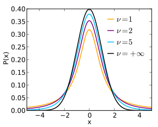
In probability and statistics, Student's t distribution is a continuous probability distribution that generalizes the standard normal distribution. Like the latter, it is symmetric around zero and bell-shaped.

<span class="mw-page-title-main">Beta distribution</span> Probability distribution

In probability theory and statistics, the beta distribution is a family of continuous probability distributions defined on the interval [0, 1] or in terms of two positive parameters, denoted by alpha (α) and beta (β), that appear as exponents of the variable and its complement to 1, respectively, and control the shape of the distribution.

In probability and statistics, a mixture distribution is the probability distribution of a random variable that is derived from a collection of other random variables as follows: first, a random variable is selected by chance from the collection according to given probabilities of selection, and then the value of the selected random variable is realized. The underlying random variables may be random real numbers, or they may be random vectors, in which case the mixture distribution is a multivariate distribution.

In statistics, a mixture model is a probabilistic model for representing the presence of subpopulations within an overall population, without requiring that an observed data set should identify the sub-population to which an individual observation belongs. Formally a mixture model corresponds to the mixture distribution that represents the probability distribution of observations in the overall population. However, while problems associated with "mixture distributions" relate to deriving the properties of the overall population from those of the sub-populations, "mixture models" are used to make statistical inferences about the properties of the sub-populations given only observations on the pooled population, without sub-population identity information.

In probability theory, a compound Poisson distribution is the probability distribution of the sum of a number of independent identically-distributed random variables, where the number of terms to be added is itself a Poisson-distributed variable. The result can be either a continuous or a discrete distribution.

<span class="mw-page-title-main">Dirichlet distribution</span> Probability distribution

In probability and statistics, the Dirichlet distribution (after Peter Gustav Lejeune Dirichlet), often denoted , is a family of continuous multivariate probability distributions parameterized by a vector of positive reals. It is a multivariate generalization of the beta distribution, hence its alternative name of multivariate beta distribution (MBD). Dirichlet distributions are commonly used as prior distributions in Bayesian statistics, and in fact, the Dirichlet distribution is the conjugate prior of the categorical distribution and multinomial distribution.

<span class="mw-page-title-main">Stable distribution</span> Distribution of variables which satisfies a stability property under linear combinations

In probability theory, a distribution is said to be stable if a linear combination of two independent random variables with this distribution has the same distribution, up to location and scale parameters. A random variable is said to be stable if its distribution is stable. The stable distribution family is also sometimes referred to as the Lévy alpha-stable distribution, after Paul Lévy, the first mathematician to have studied it.

Variational Bayesian methods are a family of techniques for approximating intractable integrals arising in Bayesian inference and machine learning. They are typically used in complex statistical models consisting of observed variables as well as unknown parameters and latent variables, with various sorts of relationships among the three types of random variables, as might be described by a graphical model. As typical in Bayesian inference, the parameters and latent variables are grouped together as "unobserved variables". Variational Bayesian methods are primarily used for two purposes:

  1. To provide an analytical approximation to the posterior probability of the unobserved variables, in order to do statistical inference over these variables.
  2. To derive a lower bound for the marginal likelihood of the observed data. This is typically used for performing model selection, the general idea being that a higher marginal likelihood for a given model indicates a better fit of the data by that model and hence a greater probability that the model in question was the one that generated the data.
<span class="mw-page-title-main">Generalized inverse Gaussian distribution</span>

In probability theory and statistics, the generalized inverse Gaussian distribution (GIG) is a three-parameter family of continuous probability distributions with probability density function

In probability theory, the Chinese restaurant process is a discrete-time stochastic process, analogous to seating customers at tables in a restaurant. Imagine a restaurant with an infinite number of circular tables, each with infinite capacity. Customer 1 sits at the first table. The next customer either sits at the same table as customer 1, or the next table. This continues, with each customer choosing to either sit at an occupied table with a probability proportional to the number of customers already there, or an unoccupied table. At time n, the n customers have been partitioned among m ≤ n tables. The results of this process are exchangeable, meaning the order in which the customers sit does not affect the probability of the final distribution. This property greatly simplifies a number of problems in population genetics, linguistic analysis, and image recognition.

In natural language processing, latent Dirichlet allocation (LDA) is a Bayesian network for modeling automatically extracted topics in textual corpora. The LDA is an example of a Bayesian topic model. In this, observations are collected into documents, and each word's presence is attributable to one of the document's topics. Each document will contain a small number of topics.

<span class="mw-page-title-main">Beta-binomial distribution</span> Discrete probability distribution

In probability theory and statistics, the beta-binomial distribution is a family of discrete probability distributions on a finite support of non-negative integers arising when the probability of success in each of a fixed or known number of Bernoulli trials is either unknown or random. The beta-binomial distribution is the binomial distribution in which the probability of success at each of n trials is not fixed but randomly drawn from a beta distribution. It is frequently used in Bayesian statistics, empirical Bayes methods and classical statistics to capture overdispersion in binomial type distributed data.

In probability theory and statistics, the Dirichlet-multinomial distribution is a family of discrete multivariate probability distributions on a finite support of non-negative integers. It is also called the Dirichlet compound multinomial distribution (DCM) or multivariate Pólya distribution. It is a compound probability distribution, where a probability vector p is drawn from a Dirichlet distribution with parameter vector , and an observation drawn from a multinomial distribution with probability vector p and number of trials n. The Dirichlet parameter vector captures the prior belief about the situation and can be seen as a pseudocount: observations of each outcome that occur before the actual data is collected. The compounding corresponds to a Pólya urn scheme. It is frequently encountered in Bayesian statistics, machine learning, empirical Bayes methods and classical statistics as an overdispersed multinomial distribution.

In probability theory and statistics, a categorical distribution is a discrete probability distribution that describes the possible results of a random variable that can take on one of K possible categories, with the probability of each category separately specified. There is no innate underlying ordering of these outcomes, but numerical labels are often attached for convenience in describing the distribution,. The K-dimensional categorical distribution is the most general distribution over a K-way event; any other discrete distribution over a size-K sample space is a special case. The parameters specifying the probabilities of each possible outcome are constrained only by the fact that each must be in the range 0 to 1, and all must sum to 1.

Financial models with long-tailed distributions and volatility clustering have been introduced to overcome problems with the realism of classical financial models. These classical models of financial time series typically assume homoskedasticity and normality cannot explain stylized phenomena such as skewness, heavy tails, and volatility clustering of the empirical asset returns in finance. In 1963, Benoit Mandelbrot first used the stable distribution to model the empirical distributions which have the skewness and heavy-tail property. Since -stable distributions have infinite -th moments for all , the tempered stable processes have been proposed for overcoming this limitation of the stable distribution.

<span class="mw-page-title-main">Poisson distribution</span> Discrete probability distribution

In probability theory and statistics, the Poisson distribution is a discrete probability distribution that expresses the probability of a given number of events occurring in a fixed interval of time if these events occur with a known constant mean rate and independently of the time since the last event. It can also be used for the number of events in other types of intervals than time, and in dimension greater than 1.

A geometric stable distribution or geo-stable distribution is a type of leptokurtic probability distribution. Geometric stable distributions were introduced in Klebanov, L. B., Maniya, G. M., and Melamed, I. A. (1985). A problem of Zolotarev and analogs of infinitely divisible and stable distributions in a scheme for summing a random number of random variables. These distributions are analogues for stable distributions for the case when the number of summands is random, independent of the distribution of summand, and having geometric distribution. The geometric stable distribution may be symmetric or asymmetric. A symmetric geometric stable distribution is also referred to as a Linnik distribution. The Laplace distribution and asymmetric Laplace distribution are special cases of the geometric stable distribution. The Mittag-Leffler distribution is also a special case of a geometric stable distribution.

In statistics and machine learning, the hierarchical Dirichlet process (HDP) is a nonparametric Bayesian approach to clustering grouped data. It uses a Dirichlet process for each group of data, with the Dirichlet processes for all groups sharing a base distribution which is itself drawn from a Dirichlet process. This method allows groups to share statistical strength via sharing of clusters across groups. The base distribution being drawn from a Dirichlet process is important, because draws from a Dirichlet process are atomic probability measures, and the atoms will appear in all group-level Dirichlet processes. Since each atom corresponds to a cluster, clusters are shared across all groups. It was developed by Yee Whye Teh, Michael I. Jordan, Matthew J. Beal and David Blei and published in the Journal of the American Statistical Association in 2006, as a formalization and generalization of the infinite hidden Markov model published in 2002.

In probability theory and statistics, the Dirichlet process (DP) is one of the most popular Bayesian nonparametric models. It was introduced by Thomas Ferguson as a prior over probability distributions.

References

  1. Frigyik, Bela A.; Kapila, Amol; Gupta, Maya R. "Introduction to the Dirichlet Distribution and Related Processes" (PDF). Retrieved 2 September 2021.
  2. Ferguson, Thomas (1973). "Bayesian analysis of some nonparametric problems". Annals of Statistics . 1 (2): 209–230. doi: 10.1214/aos/1176342360 . MR   0350949.
  3. "Dirichlet Process and Dirichlet Distribution – Polya Restaurant Scheme and Chinese Restaurant Process".
  4. For the proof, see Paisley, John (August 2010). "A simple proof of the stick-breaking construction of the Dirichlet Process" (PDF). Columbia University. Archived from the original (PDF) on January 22, 2015.
  5. Aad van der Vaart, Subhashis Ghosal (2017). Fundamentals of Bayesian Nonparametric Inference. Cambridge University Press. ISBN   978-0-521-87826-5.
  6. Sudderth, Erik (2006). Graphical Models for Visual Object Recognition and Tracking (PDF) (Ph.D.). MIT Press.
  7. Nils Lid Hjort; Chris Holmes, Peter Müller; Stephen G. Walker (2010). Bayesian Nonparametrics. Cambridge University Press. ISBN   978-0-521-51346-3.
  8. Sotirios P. Chatzis, "A Latent Variable Gaussian Process Model with Pitman-Yor Process Priors for Multiclass Classification," Neurocomputing, vol. 120, pp. 482–489, Nov. 2013. doi : 10.1016/j.neucom.2013.04.029
  9. Sotirios P. Chatzis, Yiannis Demiris, "Nonparametric mixtures of Gaussian processes with power-law behaviour," IEEE Transactions on Neural Networks and Learning Systems, vol. 23, no. 12, pp. 1862–1871, Dec. 2012. doi : 10.1109/TNNLS.2012.2217986
  10. Rasmussen, Carl (2000). "The Infinite Gaussian Mixture Model" (PDF). Advances in Neural Information Processing Systems. 12: 554–560.
  11. Sotirios P. Chatzis, Dimitrios Korkinof, and Yiannis Demiris, "A nonparametric Bayesian approach toward robot learning by demonstration," Robotics and Autonomous Systems, vol. 60, no. 6, pp. 789–802, June 2012. doi : 10.1016/j.robot.2012.02.005