In probability theory, conditional independence describes situations wherein an observation is irrelevant or redundant when evaluating the certainty of a hypothesis. Conditional independence is usually formulated in terms of conditional probability, as a special case where the probability of the hypothesis given the uninformative observation is equal to the probability without. If is the hypothesis, and and are observations, conditional independence can be stated as an equality:
where is the probability of given both and . Since the probability of given is the same as the probability of given both and , this equality expresses that contributes nothing to the certainty of . In this case, and are said to be conditionally independent given , written symbolically as: . In the language of causal equality notation, two functions and which both depend on a common variable are described as conditionally independent using the notation , which is equivalent to the notation .
The concept of conditional independence is essential to graph-based theories of statistical inference, as it establishes a mathematical relation between a collection of conditional statements and a graphoid.
Conditional independence of events
Let , , and be events. and are said to be conditionally independent given if and only if and:
This property is often written: , which should be read .
Equivalently, conditional independence may be stated as:
Each cell represents a possible outcome. The events , and are represented by the areas shaded red, blue and yellow respectively. The overlap between the events and is shaded purple.
The probabilities of these events are shaded areas with respect to the total area. In both examples and are conditionally independent given because:
Let events A and B be defined as the probability that person A and person B will be home in time for dinner where both people are randomly sampled from the entire world. Events A and B can be assumed to be independent i.e. knowledge that A is late has minimal to no change on the probability that B will be late. However, if a third event is introduced, person A and person B live in the same neighborhood, the two events are now considered not conditionally independent. Traffic conditions and weather-related events that might delay person A, might delay person B as well. Given the third event and knowledge that person A was late, the probability that person B will be late does meaningfully change.[2]
Dice rolling
Conditional independence depends on the nature of the third event. If you roll two dice, one may assume that the two dice behave independently of each other. Looking at the results of one dice will not tell you about the result of the second dice. (That is, the two dice are independent.) If, however, the 1st dice's result is a 3, and someone tells you about a third event - that the sum of the two results is even - then this extra unit of information restricts the options for the 2nd result to an odd number. In other words, two events can be independent, but NOT conditionally independent.[2]
Height and vocabulary
Height and vocabulary are dependent since very small people tend to be children, known for their more basic vocabularies. But knowing that two people are 19 years old (i.e., conditional on age) there is no reason to think that one person's vocabulary is larger if we are told that they are taller.
Conditional independence of random variables
Two discrete random variables and are conditionally independent given a third discrete random variable if and only if they are independent in their conditional probability distribution given . That is, and are conditionally independent given if and only if, given any value of , the probability distribution of is the same for all values of and the probability distribution of is the same for all values of . Formally:
Two random variables and are conditionally independent given a σ-algebra if the above equation holds for all in and in .
Two random variables and are conditionally independent given a random variable if they are independent given σ(W): the σ-algebra generated by . This is commonly written:
or
This it read " is independent of , given"; the conditioning applies to the whole statement: "( is independent of ) given ".
If assumes a countable set of values, this is equivalent to the conditional independence of X and Y for the events of the form . Conditional independence of more than two events, or of more than two random variables, is defined analogously.
The following two examples show that neither implies nor is implied by.
First, suppose is 0 with probability 0.5 and 1 otherwise. When W=0 take and to be independent, each having the value 0 with probability 0.99 and the value 1 otherwise. When , and are again independent, but this time they take the value 1 with probability 0.99. Then . But and are dependent, because Pr(X=0) < Pr(X=0|Y=0). This is because Pr(X=0) =0.5, but if Y=0 then it's very likely that W=0 and thus that X=0 as well, so Pr(X=0|Y=0)>0.5.
For the second example, suppose , each taking the values 0 and 1 with probability0.5. Let be the product . Then when , Pr(X=0)=2/3, but Pr(X=0|Y=0)=1/2, so is false. This is also an example of Explaining Away. See Kevin Murphy's tutorial [3] where and take the values "brainy" and "sporty".
Conditional independence of random vectors
Two random vectors and are conditionally independent given a third random vector if and only if they are independent in their conditional cumulative distribution given . Formally:
(Eq.3)
where , and and the conditional cumulative distributions are defined as follows.
Uses in Bayesian inference
Let p be the proportion of voters who will vote "yes" in an upcoming referendum. In taking an opinion poll, one chooses n voters randomly from the population. For i=1,...,n, let Xi=1 or 0 corresponding, respectively, to whether or not the ith chosen voter will or will not vote "yes".
In a frequentist approach to statistical inference one would not attribute any probability distribution to p (unless the probabilities could be somehow interpreted as relative frequencies of occurrence of some event or as proportions of some population) and one would say that X1, ..., Xn are independent random variables.
By contrast, in a Bayesian approach to statistical inference, one would assign a probability distribution to p regardless of the non-existence of any such "frequency" interpretation, and one would construe the probabilities as degrees of belief that p is in any interval to which a probability is assigned. In that model, the random variables X1,...,Xn are not independent, but they are conditionally independent given the value of p. In particular, if a large number of the Xs are observed to be equal to 1, that would imply a high conditional probability, given that observation, that p is near 1, and thus a high conditional probability, given that observation, that the nextX to be observed will be equal to 1.
Rules of conditional independence
A set of rules governing statements of conditional independence have been derived from the basic definition.[4][5]
These rules were termed "Graphoid Axioms" by Pearl and Paz,[6] because they hold in graphs, where is interpreted to mean: "All paths from X to A are intercepted by the set B".[7]
Symmetry
Decomposition
Proof
(meaning of )
(ignore variable B by integrating it out)
A similar proof shows the independence of X and B.
Weak union
Proof
By assumption, .
Due to the property of decomposition , .
Combining the above two equalities gives , which establishes .
The second condition can be proved similarly.
Contraction
Proof
This property can be proved by noticing , each equality of which is asserted by and , respectively.
Intersection
For strictly positive probability distributions,[5] the following also holds:
Technical note: since these implications hold for any probability space, they will still hold if one considers a sub-universe by conditioning everything on another variable, sayK. For example, would also mean that .
In probability theory and statistics, the cumulative distribution function (CDF) of a real-valued random variable , or just distribution function of , evaluated at , is the probability that will take a value less than or equal to .
Independence is a fundamental notion in probability theory, as in statistics and the theory of stochastic processes. Two events are independent, statistically independent, or stochastically independent if, informally speaking, the occurrence of one does not affect the probability of occurrence of the other or, equivalently, does not affect the odds. Similarly, two random variables are independent if the realization of one does not affect the probability distribution of the other.
In probability theory, the central limit theorem (CLT) establishes that, in many situations, for independent and identically distributed random variables, the sampling distribution of the standardized sample mean tends towards the standard normal distribution even if the original variables themselves are not normally distributed.
In probability theory, a probability density function (PDF), density function, or density of an absolutely continuous random variable, is a function whose value at any given sample in the sample space can be interpreted as providing a relative likelihood that the value of the random variable would be equal to that sample. Probability density is the probability per unit length, in other words, while the absolute likelihood for a continuous random variable to take on any particular value is 0, the value of the PDF at two different samples can be used to infer, in any particular draw of the random variable, how much more likely it is that the random variable would be close to one sample compared to the other sample.
In probability theory and statistics, the multivariate normal distribution, multivariate Gaussian distribution, or joint normal distribution is a generalization of the one-dimensional (univariate) normal distribution to higher dimensions. One definition is that a random vector is said to be k-variate normally distributed if every linear combination of its k components has a univariate normal distribution. Its importance derives mainly from the multivariate central limit theorem. The multivariate normal distribution is often used to describe, at least approximately, any set of (possibly) correlated real-valued random variables each of which clusters around a mean value.
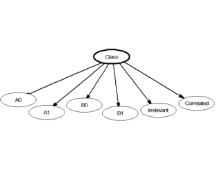
In statistics, naive Bayes classifiers are a family of linear "probabilistic classifiers" based on applying Bayes' theorem with strong (naive) independence assumptions between the features. They are among the simplest Bayesian network models, but coupled with kernel density estimation, they can achieve high accuracy levels.
In statistics, a statistic is sufficient with respect to a statistical model and its associated unknown parameter if "no other statistic that can be calculated from the same sample provides any additional information as to the value of the parameter". In particular, a statistic is sufficient for a family of probability distributions if the sample from which it is calculated gives no additional information than the statistic, as to which of those probability distributions is the sampling distribution.
In probability theory and statistics, two real-valued random variables, , , are said to be uncorrelated if their covariance, , is zero. If two variables are uncorrelated, there is no linear relationship between them.
In probability theory and statistics, a covariance matrix is a square matrix giving the covariance between each pair of elements of a given random vector.
In probability theory, a martingale is a sequence of random variables for which, at a particular time, the conditional expectation of the next value in the sequence is equal to the present value, regardless of all prior values.
In linear algebra and functional analysis, a projection is a linear transformation from a vector space to itself such that . That is, whenever is applied twice to any vector, it gives the same result as if it were applied once. It leaves its image unchanged. This definition of "projection" formalizes and generalizes the idea of graphical projection. One can also consider the effect of a projection on a geometrical object by examining the effect of the projection on points in the object.
Given two random variables that are defined on the same probability space, the joint probability distribution is the corresponding probability distribution on all possible pairs of outputs. The joint distribution can just as well be considered for any given number of random variables. The joint distribution encodes the marginal distributions, i.e. the distributions of each of the individual random variables. It also encodes the conditional probability distributions, which deal with how the outputs of one random variable are distributed when given information on the outputs of the other random variable(s).
Probability theory and statistics have some commonly used conventions, in addition to standard mathematical notation and mathematical symbols.
In mathematics, Schubert calculus is a branch of algebraic geometry introduced in the nineteenth century by Hermann Schubert, in order to solve various counting problems of projective geometry. It was a precursor of several more modern theories, for example characteristic classes, and in particular its algorithmic aspects are still of current interest. The term Schubert calculus is sometimes used to mean the enumerative geometry of linear subspaces of a vector space, which is roughly equivalent to describing the cohomology ring of Grassmannians. Sometimes it is used to mean the more general enumerative geometry of algebraic varieties that are homogenous spaces of simple Lie groups. Even more generally, Schubert calculus is often understood to encompass the study of analogous questions in generalized cohomology theories.
In mathematics, a π-system on a set is a collection of certain subsets of such that
In statistics, an exchangeable sequence of random variables is a sequence X1, X2, X3, ... whose joint probability distribution does not change when the positions in the sequence in which finitely many of them appear are altered. Thus, for example the sequences
Bayesian linear regression is a type of conditional modeling in which the mean of one variable is described by a linear combination of other variables, with the goal of obtaining the posterior probability of the regression coefficients and ultimately allowing the out-of-sample prediction of the regressandconditional on observed values of the regressors. The simplest and most widely used version of this model is the normal linear model, in which given is distributed Gaussian. In this model, and under a particular choice of prior probabilities for the parameters—so-called conjugate priors—the posterior can be found analytically. With more arbitrarily chosen priors, the posteriors generally have to be approximated.
The Brownian motion models for financial markets are based on the work of Robert C. Merton and Paul A. Samuelson, as extensions to the one-period market models of Harold Markowitz and William F. Sharpe, and are concerned with defining the concepts of financial assets and markets, portfolios, gains and wealth in terms of continuous-time stochastic processes.
In probability theory and statistics, the generalized chi-squared distribution is the distribution of a quadratic form of a multinormal variable, or a linear combination of different normal variables and squares of normal variables. Equivalently, it is also a linear sum of independent noncentral chi-square variables and a normal variable. There are several other such generalizations for which the same term is sometimes used; some of them are special cases of the family discussed here, for example the gamma distribution.
For certain applications in linear algebra, it is useful to know properties of the probability distribution of the largest eigenvalue of a finite sum of random matrices. Suppose is a finite sequence of random matrices. Analogous to the well-known Chernoff bound for sums of scalars, a bound on the following is sought for a given parameter t:
References
↑ To see that this is the case, one needs to realise that Pr(R ∩ B | Y) is the probability of an overlap of R and B (the purple shaded area) in the Y area. Since, in the picture on the left, there are two squares where R and B overlap within the Y area, and the Y area has twelve squares, Pr(R ∩ B | Y) = 2/12 = 1/6. Similarly, Pr(R | Y) = 4/12 = 1/3 and Pr(B | Y) = 6/12 = 1/2.
This page is based on this Wikipedia article Text is available under the CC BY-SA 4.0 license; additional terms may apply. Images, videos and audio are available under their respective licenses.