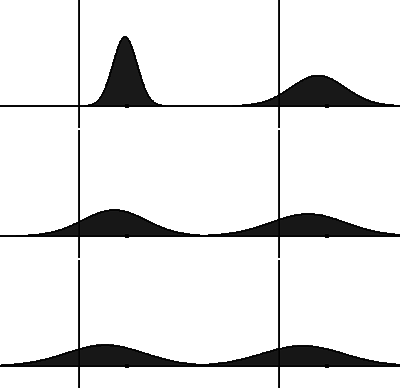
In statistical mechanics and information theory, the Fokker–Planck equation is a partial differential equation that describes the time evolution of the probability density function of the velocity of a particle under the influence of drag forces and random forces, as in Brownian motion. The equation can be generalized to other observables as well. The Fokker-Planck equation has multiple applications in information theory, graph theory, data science, finance, economics etc.

A geometric Brownian motion (GBM) (also known as exponential Brownian motion) is a continuous-time stochastic process in which the logarithm of the randomly varying quantity follows a Brownian motion (also called a Wiener process) with drift. It is an important example of stochastic processes satisfying a stochastic differential equation (SDE); in particular, it is used in mathematical finance to model stock prices in the Black–Scholes model.

In probability theory and statistics, the Rayleigh distribution is a continuous probability distribution for nonnegative-valued random variables. Up to rescaling, it coincides with the chi distribution with two degrees of freedom. The distribution is named after Lord Rayleigh.
A stochastic differential equation (SDE) is a differential equation in which one or more of the terms is a stochastic process, resulting in a solution which is also a stochastic process. SDEs have many applications throughout pure mathematics and are used to model various behaviours of stochastic models such as stock prices, random growth models or physical systems that are subjected to thermal fluctuations.
In thermodynamics, an activity coefficient is a factor used to account for deviation of a mixture of chemical substances from ideal behaviour. In an ideal mixture, the microscopic interactions between each pair of chemical species are the same and, as a result, properties of the mixtures can be expressed directly in terms of simple concentrations or partial pressures of the substances present e.g. Raoult's law. Deviations from ideality are accommodated by modifying the concentration by an activity coefficient. Analogously, expressions involving gases can be adjusted for non-ideality by scaling partial pressures by a fugacity coefficient.
In probability theory and statistics, the generalized extreme value (GEV) distribution is a family of continuous probability distributions developed within extreme value theory to combine the Gumbel, Fréchet and Weibull families also known as type I, II and III extreme value distributions. By the extreme value theorem the GEV distribution is the only possible limit distribution of properly normalized maxima of a sequence of independent and identically distributed random variables. Note that a limit distribution needs to exist, which requires regularity conditions on the tail of the distribution. Despite this, the GEV distribution is often used as an approximation to model the maxima of long (finite) sequences of random variables.

In mathematics, the Ornstein–Uhlenbeck process is a stochastic process with applications in financial mathematics and the physical sciences. Its original application in physics was as a model for the velocity of a massive Brownian particle under the influence of friction. It is named after Leonard Ornstein and George Eugene Uhlenbeck.
In statistics, stochastic volatility models are those in which the variance of a stochastic process is itself randomly distributed. They are used in the field of mathematical finance to evaluate derivative securities, such as options. The name derives from the models' treatment of the underlying security's volatility as a random process, governed by state variables such as the price level of the underlying security, the tendency of volatility to revert to some long-run mean value, and the variance of the volatility process itself, among others.
The normal-inverse Gaussian distribution is a continuous probability distribution that is defined as the normal variance-mean mixture where the mixing density is the inverse Gaussian distribution. The NIG distribution was noted by Blaesild in 1977 as a subclass of the generalised hyperbolic distribution discovered by Ole Barndorff-Nielsen. In the next year Barndorff-Nielsen published the NIG in another paper. It was introduced in the mathematical finance literature in 1997.
In mathematics, Gaussian measure is a Borel measure on finite-dimensional Euclidean space , closely related to the normal distribution in statistics. There is also a generalization to infinite-dimensional spaces. Gaussian measures are named after the German mathematician Carl Friedrich Gauss. One reason why Gaussian measures are so ubiquitous in probability theory is the central limit theorem. Loosely speaking, it states that if a random variable is obtained by summing a large number of independent random variables with variance 1, then has variance and its law is approximately Gaussian.
In mathematical finance, the SABR model is a stochastic volatility model, which attempts to capture the volatility smile in derivatives markets. The name stands for "stochastic alpha, beta, rho", referring to the parameters of the model. The SABR model is widely used by practitioners in the financial industry, especially in the interest rate derivative markets. It was developed by Patrick S. Hagan, Deep Kumar, Andrew Lesniewski, and Diana Woodward.
A local volatility model, in mathematical finance and financial engineering, is an option pricing model that treats volatility as a function of both the current asset level and of time . As such, it is a generalisation of the Black–Scholes model, where the volatility is a constant. Local volatility models are often compared with stochastic volatility models, where the instantaneous volatility is not just a function of the asset level but depends also on a new "global" randomness coming from an additional random component.
The Birnbaum–Saunders distribution, also known as the fatigue life distribution, is a probability distribution used extensively in reliability applications to model failure times. There are several alternative formulations of this distribution in the literature. It is named after Z. W. Birnbaum and S. C. Saunders.
Financial models with long-tailed distributions and volatility clustering have been introduced to overcome problems with the realism of classical financial models. These classical models of financial time series typically assume homoskedasticity and normality cannot explain stylized phenomena such as skewness, heavy tails, and volatility clustering of the empirical asset returns in finance. In 1963, Benoit Mandelbrot first used the stable distribution to model the empirical distributions which have the skewness and heavy-tail property. Since -stable distributions have infinite -th moments for all , the tempered stable processes have been proposed for overcoming this limitation of the stable distribution.

In the theory of stochastic processes, a part of the mathematical theory of probability, the variance gamma (VG) process, also known as Laplace motion, is a Lévy process determined by a random time change. The process has finite moments, distinguishing it from many Lévy processes. There is no diffusion component in the VG process and it is thus a pure jump process. The increments are independent and follow a variance-gamma distribution, which is a generalization of the Laplace distribution.
In financial econometrics, the Markov-switching multifractal (MSM) is a model of asset returns developed by Laurent E. Calvet and Adlai J. Fisher that incorporates stochastic volatility components of heterogeneous durations. MSM captures the outliers, log-memory-like volatility persistence and power variation of financial returns. In currency and equity series, MSM compares favorably with standard volatility models such as GARCH(1,1) and FIGARCH both in- and out-of-sample. MSM is used by practitioners in the financial industry to forecast volatility, compute value-at-risk, and price derivatives.
In probability theory and statistics, the normal-inverse-Wishart distribution is a multivariate four-parameter family of continuous probability distributions. It is the conjugate prior of a multivariate normal distribution with unknown mean and covariance matrix.
In probability theory, a subordinator is a stochastic process that is non-negative and whose increments are stationary and independent. Subordinators are a special class of Lévy process that play an important role in the theory of local time. In this context, subordinators describe the evolution of time within another stochastic process, the subordinated stochastic process. In other words, a subordinator will determine the random number of "time steps" that occur within the subordinated process for a given unit of chronological time.
An additive process, in probability theory, is a cadlag, continuous in probability stochastic process with independent increments. An additive process is the generalization of a Lévy process. An example of an additive process that is not a Lévy process is a Brownian motion with a time-dependent drift. The additive process was introduced by Paul Lévy in 1937.
A mixed Poisson distribution is a univariate discrete probability distribution in stochastics. It results from assuming that the conditional distribution of a random variable, given the value of the rate parameter, is a Poisson distribution, and that the rate parameter itself is considered as a random variable. Hence it is a special case of a compound probability distribution. Mixed Poisson distributions can be found in actuarial mathematics as a general approach for the distribution of the number of claims and is also examined as an epidemiological model. It should not be confused with compound Poisson distribution or compound Poisson process.


