Moran process

Last updated

A Moran process or Moran model is a simple stochastic process used in biology to describe finite populations. The process is named after Patrick Moran, who first proposed the model in 1958. [1] It can be used to model variety-increasing processes such as mutation as well as variety-reducing effects such as genetic drift and natural selection. The process can describe the probabilistic dynamics in a finite population of constant size N in which two alleles A and B are competing for dominance. The two alleles are considered to be true replicators (i.e. entities that make copies of themselves).

Contents

In each time step a random individual (which is of either type A or B) is chosen for reproduction and a random individual is chosen for death; thus ensuring that the population size remains constant. To model selection, one type has to have a higher fitness and is thus more likely to be chosen for reproduction. The same individual can be chosen for death and for reproduction in the same step.

Neutral drift

Neutral drift is the idea that a neutral mutation can spread throughout a population, so that eventually the original allele is lost. A neutral mutation does not bring any fitness advantage or disadvantage to its bearer. The simple case of the Moran process can describe this phenomenon.

The Moran process is defined on the state space i = 0, ..., N which count the number of A individuals. Since the number of A individuals can change at most by one at each time step, a transition exists only between state i and state i − 1, i and i + 1. Thus the transition matrix of the stochastic process is tri-diagonal in shape and the transition probabilities are

The entry denotes the probability to go from state i to state j. To understand the formulas for the transition probabilities one has to look at the definition of the process which states that always one individual will be chosen for reproduction and one is chosen for death. Once the A individuals have died out, they will never be reintroduced into the population since the process does not model mutations (A cannot be reintroduced into the population once it has died out and vice versa) and thus . For the same reason the population of A individuals will always stay N once they have reached that number and taken over the population and thus . The states 0 and N are called absorbing while the states 1, ..., N − 1 are called transient. The intermediate transition probabilities can be explained by considering the first term to be the probability to choose the individual whose abundance will increase by one and the second term the probability to choose the other type for death. Obviously, if the same type is chosen for reproduction and for death, then the abundance of one type does not change.

Eventually the population will reach one of the absorbing states and then stay there forever. In the transient states, random fluctuations will occur but eventually the population of A will either go extinct or reach fixation. This is one of the most important differences to deterministic processes which cannot model random events. The expected value and the variance of the number of A individuals X(t) at timepoint t can be computed when an initial state X(0) = i is given:

For a mathematical derivation of the equation above, click on "show" to reveal

For the expected value the calculation runs as follows. Writing p = i/N,

Writing and , and applying the law of total expectation, Applying the argument repeatedly gives or

For the variance the calculation runs as follows. Writing we have

For all t, and are identically distributed, so their variances are equal. Writing as before and , and applying the law of total variance,

If , we obtain

Rewriting this equation as

yields

as desired.


The probability that A reaches fixation is called fixation probability. For the simple Moran process this probability is xi = i/N.

Since all individuals have the same fitness, they also have the same chance of becoming the ancestor of the whole population; this probability is 1/N and thus the sum of all i probabilities (for all A individuals) is just i/N. The mean time to absorption starting in state i is given by

For a mathematical derivation of the equation above, click on "show" to reveal

The mean time spent in state j when starting in state i which is given by

Here δij denotes the Kroenecker delta. This recursive equation can be solved using a new variable qi so that and thus and rewritten

The variable is used and the equation becomes

Knowing that and

we can calculate :

Therefore

with . Now ki, the total time until fixation starting from state i, can be calculated


For large N the approximation

holds.

Selection

If one allele has a fitness advantage over the other allele, it will be more likely to be chosen for reproduction. This can be incorporated into the model if individuals with allele A have fitness and individuals with allele B have fitness where is the number of individuals of type A; thus describing a general birth-death process. The transition matrix of the stochastic process is tri-diagonal in shape. Let , then the transition probabilities are

The entry denotes the probability to go from state i to state j. The difference to neutral selection above is now that reproduction of an individual with allele B is accepted with probability

and reproduction of an individual with allele A is accepted with probability

when the number of individuals with allele B is exactly i.

Also in this case, fixation probabilities when starting in state i is defined by recurrence

And the closed form is given by

where per definition and will just be for the general case.

For a mathematical derivation of the equation above, click on "show" to reveal

Also in this case, fixation probabilities can be computed, but the transition probabilities are not symmetric. The notation and is used. The fixation probability can be defined recursively and a new variable is introduced.

Now two properties from the definition of the variable yi can be used to find a closed form solution for the fixation probabilities:

Combining (3) and xN = 1:

which implies:

This in turn gives us:


This general case where the fitness of A and B depends on the abundance of each type is studied in evolutionary game theory.

Less complex results are obtained if a constant fitness ratio , for all i, is assumed. Individuals of type A reproduce with a constant rate r and individuals with allele B reproduce with rate 1. Thus if A has a fitness advantage over B, r will be larger than one, otherwise it will be smaller than one. Thus the transition matrix of the stochastic process is tri-diagonal in shape and the transition probabilities are

In this case is a constant factor for each composition of the population and thus the fixation probability from equation (1) simplifies to

where the fixation probability of a single mutant A in a population of otherwise all B is often of interest and is denoted by ρ.

Also in the case of selection, the expected value and the variance of the number of A individuals may be computed

where p = i/N, and r = 1 + s.

For a mathematical derivation of the equation above, click on "show" to reveal

For the expected value the calculation runs as follows

For the variance the calculation runs as follows, using the variance of a single step


Rate of evolution

In a population of all B individuals, a single mutant A will take over the whole population with the probability

If the mutation rate (to go from the B to the A allele) in the population is u then the rate with which one member of the population will mutate to A is given by N × u and the rate with which the whole population goes from all B to all A is the rate that a single mutant A arises times the probability that it will take over the population (fixation probability):

Thus if the mutation is neutral (i.e. the fixation probability is just 1/N) then the rate with which an allele arises and takes over a population is independent of the population size and is equal to the mutation rate. This important result is the basis of the neutral theory of evolution and suggests that the number of observed point mutations in the genomes of two different species would simply be given by the mutation rate multiplied by two times the time since divergence. Thus the neutral theory of evolution provides a molecular clock, given that the assumptions are fulfilled which may not be the case in reality.

See also

Related Research Articles

<span class="mw-page-title-main">Variance</span> Statistical measure of how far values spread from their average

In probability theory and statistics, variance is the expected value of the squared deviation from the mean of a random variable. The standard deviation (SD) is obtained as the square root of the variance. Variance is a measure of dispersion, meaning it is a measure of how far a set of numbers is spread out from their average value. It is the second central moment of a distribution, and the covariance of the random variable with itself, and it is often represented by , , , , or .

The weighted arithmetic mean is similar to an ordinary arithmetic mean, except that instead of each of the data points contributing equally to the final average, some data points contribute more than others. The notion of weighted mean plays a role in descriptive statistics and also occurs in a more general form in several other areas of mathematics.

<span class="mw-page-title-main">Geometric distribution</span> Probability distribution

In probability theory and statistics, the geometric distribution is either one of two discrete probability distributions:

<span class="mw-page-title-main">Log-normal distribution</span> Probability distribution

In probability theory, a log-normal (or lognormal) distribution is a continuous probability distribution of a random variable whose logarithm is normally distributed. Thus, if the random variable X is log-normally distributed, then Y = ln(X) has a normal distribution. Equivalently, if Y has a normal distribution, then the exponential function of Y, X = exp(Y), has a log-normal distribution. A random variable which is log-normally distributed takes only positive real values. It is a convenient and useful model for measurements in exact and engineering sciences, as well as medicine, economics and other topics (e.g., energies, concentrations, lengths, prices of financial instruments, and other metrics).

Covariance in probability theory and statistics is a measure of the joint variability of two random variables.

In mathematics, a generating function is a representation of an infinite sequence of numbers as the coefficients of a formal power series. Unlike an ordinary series, the formal power series is not required to converge: in fact, the generating function is not actually regarded as a function, and the "variable" remains an indeterminate. Generating functions were first introduced by Abraham de Moivre in 1730, in order to solve the general linear recurrence problem. One can generalize to formal power series in more than one indeterminate, to encode information about infinite multi-dimensional arrays of numbers.

<span class="mw-page-title-main">Error function</span> Sigmoid shape special function

In mathematics, the error function, often denoted by erf, is a function defined as:

<span class="mw-page-title-main">Logistic regression</span> Statistical model for a binary dependent variable

In statistics, the logistic model is a statistical model that models the log-odds of an event as a linear combination of one or more independent variables. In regression analysis, logistic regression is estimating the parameters of a logistic model. Formally, in binary logistic regression there is a single binary dependent variable, coded by an indicator variable, where the two values are labeled "0" and "1", while the independent variables can each be a binary variable or a continuous variable. The corresponding probability of the value labeled "1" can vary between 0 and 1, hence the labeling; the function that converts log-odds to probability is the logistic function, hence the name. The unit of measurement for the log-odds scale is called a logit, from logistic unit, hence the alternative names. See § Background and § Definition for formal mathematics, and § Example for a worked example.

In probability theory, the probability generating function of a discrete random variable is a power series representation (the generating function) of the probability mass function of the random variable. Probability generating functions are often employed for their succinct description of the sequence of probabilities Pr(X = i) in the probability mass function for a random variable X, and to make available the well-developed theory of power series with non-negative coefficients.

In mathematics, a Gaussian function, often simply referred to as a Gaussian, is a function of the base form

In probability theory and statistics, the cumulantsκn of a probability distribution are a set of quantities that provide an alternative to the moments of the distribution. Any two probability distributions whose moments are identical will have identical cumulants as well, and vice versa.

The Basel problem is a problem in mathematical analysis with relevance to number theory, concerning an infinite sum of inverse squares. It was first posed by Pietro Mengoli in 1650 and solved by Leonhard Euler in 1734, and read on 5 December 1735 in The Saint Petersburg Academy of Sciences. Since the problem had withstood the attacks of the leading mathematicians of the day, Euler's solution brought him immediate fame when he was twenty-eight. Euler generalised the problem considerably, and his ideas were taken up more than a century later by Bernhard Riemann in his seminal 1859 paper "On the Number of Primes Less Than a Given Magnitude", in which he defined his zeta function and proved its basic properties. The problem is named after Basel, hometown of Euler as well as of the Bernoulli family who unsuccessfully attacked the problem.

<span class="mw-page-title-main">Buffon's needle problem</span> Question in geometric probability

In probability theory, Buffon's needle problem is a question first posed in the 18th century by Georges-Louis Leclerc, Comte de Buffon:

In probability theory, a compound Poisson distribution is the probability distribution of the sum of a number of independent identically-distributed random variables, where the number of terms to be added is itself a Poisson-distributed variable. The result can be either a continuous or a discrete distribution.

In probability theory, the multinomial distribution is a generalization of the binomial distribution. For example, it models the probability of counts for each side of a k-sided dice rolled n times. For n independent trials each of which leads to a success for exactly one of k categories, with each category having a given fixed success probability, the multinomial distribution gives the probability of any particular combination of numbers of successes for the various categories.

In queueing theory, a discipline within the mathematical theory of probability, a Jackson network is a class of queueing network where the equilibrium distribution is particularly simple to compute as the network has a product-form solution. It was the first significant development in the theory of networks of queues, and generalising and applying the ideas of the theorem to search for similar product-form solutions in other networks has been the subject of much research, including ideas used in the development of the Internet. The networks were first identified by James R. Jackson and his paper was re-printed in the journal Management Science’s ‘Ten Most Influential Titles of Management Sciences First Fifty Years.’

In natural language processing, latent Dirichlet allocation (LDA) is a Bayesian network for modeling automatically extracted topics in textual corpora. The LDA is an example of a Bayesian topic model. In this, observations are collected into documents, and each word's presence is attributable to one of the document's topics. Each document will contain a small number of topics.

<span class="mw-page-title-main">Coupon collector's problem</span> Problem in probability theory

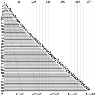
In probability theory, the coupon collector's problem refers to mathematical analysis of "collect all coupons and win" contests. It asks the following question: If each box of a brand of cereals contains a coupon, and there are n different types of coupons, what is the probability that more than t boxes need to be bought to collect all n coupons? An alternative statement is: Given n coupons, how many coupons do you expect you need to draw with replacement before having drawn each coupon at least once? The mathematical analysis of the problem reveals that the expected number of trials needed grows as . For example, when n = 50 it takes about 225 trials on average to collect all 50 coupons.

The purpose of this page is to provide supplementary materials for the ordinary least squares article, reducing the load of the main article with mathematics and improving its accessibility, while at the same time retaining the completeness of exposition.

References

  1. Moran, P. A. P. (1958). "Random processes in genetics". Mathematical Proceedings of the Cambridge Philosophical Society . 54 (1): 60–71. doi:10.1017/S0305004100033193.

Further reading