Divergence

This article is about divergence in vector calculus. For divergence of infinite series, see Divergent series. For divergence in statistics, see Divergence (statistics). For other uses, see Divergence (disambiguation).

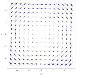
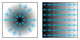
The divergence of different vector fields. The divergence of vectors from point (x,y) equals the sum of the partial derivative-with-respect-to-x of the x-component and the partial derivative-with-respect-to-y of the y-component at that point: ${\displaystyle \nabla \!\cdot (\mathbf {V} (x,y))={\frac {\partial \,{V_{x}(x,y)}}{\partial {x}}}+{\frac {\partial \,{V_{y}(x,y)}}{\partial {y}}}}$

In vector calculus, divergence is a vector operator that operates on a vector field, producing a scalar field giving the quantity of the vector field's source at each point. More technically, the divergence represents the volume density of the outward flux of a vector field from an infinitesimal volume around a given point.

As an example, consider air as it is heated or cooled. The velocity of the air at each point defines a vector field. While air is heated in a region, it expands in all directions, and thus the velocity field points outward from that region. The divergence of the velocity field in that region would thus have a positive value. While the air is cooled and thus contracting, the divergence of the velocity has a negative value.

Physical interpretation of divergence

In physical terms, the divergence of a vector field is the extent to which the vector field flux behaves like a source at a given point. It is a local measure of its "outgoingness" – the extent to which there are more of the field vectors exiting from an infinitesimal region of space than entering it. A point at which the flux is outgoing has positive divergence, and is often called a "source" of the field. A point at which the flux is directed inward has negative divergence, and is often called a "sink" of the field. The greater the flux of field through a small surface enclosing a given point, the greater the value of divergence at that point. A point at which there is zero flux through an enclosing surface has zero divergence.

The divergence of a vector field is often illustrated using the simple example of the velocity field of a fluid, a liquid or gas. A moving gas has a velocity, a speed and direction at each point, which can be represented by a vector, so the velocity of the gas forms a vector field. If a gas is heated, it will expand. This will cause a net motion of gas particles outward in all directions. Any closed surface in the gas will enclose gas which is expanding, so there will be an outward flux of gas through the surface. So the velocity field will have positive divergence everywhere. Similarly, if the gas is cooled, it will contract. There will be more room for gas particles in any volume, so the external pressure of the fluid will cause a net flow of gas volume inward through any closed surface. Therefore the velocity field has negative divergence everywhere. In contrast, in a gas at a constant temperature and pressure, the net flux of gas out of any closed surface is zero. The gas may be moving, but the volume rate of gas flowing into any closed surface must equal the volume rate flowing out, so the net flux is zero. Thus the gas velocity has zero divergence everywhere. A field which has zero divergence everywhere is called solenoidal.

If the gas is heated only at one point or small region, or a small tube is introduced which supplies a source of additional gas at one point, the gas there will expand, pushing fluid particles around it outward in all directions. This will cause an outward velocity field throughout the gas, centered on the heated point. Any closed surface enclosing the heated point will have a flux of gas particles passing out of it, so there is positive divergence at that point. However any closed surface not enclosing the point will have a constant density of gas inside, so just as many fluid particles are entering as leaving the volume, thus the net flux out of the volume is zero. Therefore the divergence at any other point is zero.

Definition

The divergence at a point x is the limit of the ratio of the flux ${\displaystyle \Phi }$ through the surface S_i(red arrows) to the volume ${\displaystyle |V_{i}|}$ for any sequence of closed regions V₁, V₂, V₃, … enclosing x that approaches zero volume:
${\displaystyle \operatorname {div} \mathbf {F} =\lim _{|V_{i}|\to 0}{\frac {\Phi (S_{i})}{|V_{i}|}}}$

The divergence of a vector field F(x) at a point x₀ is defined as the limit of the ratio of the surface integral of F out of the closed surface of a volume V enclosing x₀ to the volume of V, as V shrinks to zero

${\displaystyle \left.\operatorname {div} \mathbf {F} \right|_{\mathbf {x_{0}} }=\lim _{V\to 0}{\frac {1}{|V|}}}$${\displaystyle \scriptstyle S(V)}$${\displaystyle \mathbf {F} \cdot \mathbf {\hat {n}} \,dS}$

where |V| is the volume of V, S(V) is the boundary of V, and ${\displaystyle \mathbf {\hat {n}} }$ is the outward unit normal to that surface. It can be shown that the above limit always converges to the same value for any sequence of volumes that contain x₀ and approach zero volume. The result, div F, is a scalar function of x.

Since this definition is coordinate-free, it shows that the divergence is the same in any coordinate system. However it is not often used practically to calculate divergence; when the vector field is given in a coordinate system the coordinate definitions below are much simpler to use.

A vector field with zero divergence everywhere is called solenoidal – in which case any closed surface has no net flux across it.

Definition in coordinates

Cartesian coordinates

In three-dimensional Cartesian coordinates, the divergence of a continuously differentiable vector field ${\displaystyle \mathbf {F} =F_{x}\mathbf {i} +F_{y}\mathbf {j} +F_{z}\mathbf {k} }$ is defined as the scalar-valued function:

${\displaystyle \operatorname {div} \mathbf {F} =\nabla \cdot \mathbf {F} =\left({\frac {\partial }{\partial x}},{\frac {\partial }{\partial y}},{\frac {\partial }{\partial z}}\right)\cdot (F_{x},F_{y},F_{z})={\frac {\partial F_{x}}{\partial x}}+{\frac {\partial F_{y}}{\partial y}}+{\frac {\partial F_{z}}{\partial z}}.}$

Although expressed in terms of coordinates, the result is invariant under rotations, as the physical interpretation suggests. This is because the trace of the Jacobian matrix of an N-dimensional vector field F in N-dimensional space is invariant under any invertible linear transformation^{[ clarification needed ]}.

The common notation for the divergence ∇ · F is a convenient mnemonic, where the dot denotes an operation reminiscent of the dot product: take the components of the ∇ operator (see del), apply them to the corresponding components of F, and sum the results. Because applying an operator is different from multiplying the components, this is considered an abuse of notation.

Cylindrical coordinates

For a vector expressed in local unit cylindrical coordinates as

${\displaystyle \mathbf {F} =\mathbf {e} _{r}F_{r}+\mathbf {e} _{\theta }F_{\theta }+\mathbf {e} _{z}F_{z},}$

where e_a is the unit vector in direction a, the divergence is ^[1]

${\displaystyle \operatorname {div} \mathbf {F} =\nabla \cdot \mathbf {F} ={\frac {1}{r}}{\frac {\partial }{\partial r}}\left(rF_{r}\right)+{\frac {1}{r}}{\frac {\partial F_{\theta }}{\partial \theta }}+{\frac {\partial F_{z}}{\partial z}}.}$

The use of local coordinates is vital for the validity of the expression. If we consider x the position vector and the functions r(x), θ(x), and z(x), which assign the corresponding global cylindrical coordinate to a vector, in general ${\displaystyle r(\mathbf {F} (\mathbf {x} ))\neq F_{r}(\mathbf {x} )}$, ${\displaystyle \theta (\mathbf {F} (\mathbf {x} ))\neq F_{\theta }(\mathbf {x} )}$, and ${\displaystyle z(\mathbf {F} (\mathbf {x} ))\neq F_{z}(\mathbf {x} )}$. In particular, if we consider the identity function F(x) = x, we find that:

${\displaystyle \theta (\mathbf {F} (\mathbf {x} ))=\theta \neq F_{\theta }(\mathbf {x} )=0}$.

Spherical coordinates

In spherical coordinates, with θ the angle with the z axis and φ the rotation around the z axis, and F again written in local unit coordinates, the divergence is ^[2]

${\displaystyle \operatorname {div} \mathbf {F} =\nabla \cdot \mathbf {F} ={\frac {1}{r^{2}}}{\frac {\partial }{\partial r}}\left(r^{2}F_{r}\right)+{\frac {1}{r\sin \theta }}{\frac {\partial }{\partial \theta }}(\sin \theta \,F_{\theta })+{\frac {1}{r\sin \theta }}{\frac {\partial F_{\varphi }}{\partial \varphi }}.}$

Tensor field

Let A be continuously differentiable second-order tensor field defined as follows:

${\displaystyle \mathbf {A} ={\begin{bmatrix}A_{11}&A_{12}&A_{13}\\A_{21}&A_{22}&A_{23}\\A_{31}&A_{32}&A_{33}\end{bmatrix}}}$

the divergence in cartesian coordinate system is a first-order tensor field ^[3] and can be defined in two ways: ^[4]

${\displaystyle \operatorname {div} (\mathbf {A} )={\cfrac {\partial A_{ik}}{\partial x_{k}}}~\mathbf {e} _{i}=A_{ik,k}~\mathbf {e} _{i}={\begin{bmatrix}{\dfrac {\partial A_{11}}{\partial x_{1}}}+{\dfrac {\partial A_{12}}{\partial x_{2}}}+{\dfrac {\partial A_{13}}{\partial x_{3}}}\\{\dfrac {\partial A_{21}}{\partial x_{1}}}+{\dfrac {\partial A_{22}}{\partial x_{2}}}+{\dfrac {\partial A_{23}}{\partial x_{3}}}\\{\dfrac {\partial A_{31}}{\partial x_{1}}}+{\dfrac {\partial A_{32}}{\partial x_{2}}}+{\dfrac {\partial A_{33}}{\partial x_{3}}}\end{bmatrix}}}$

and ^{[5] [6] [7]}

${\displaystyle \nabla \cdot \mathbf {A} ={\cfrac {\partial A_{ki}}{\partial x_{k}}}~\mathbf {e} _{i}=A_{ki,k}~\mathbf {e} _{i}={\begin{bmatrix}{\dfrac {\partial A_{11}}{\partial x_{1}}}+{\dfrac {\partial A_{21}}{\partial x_{2}}}+{\dfrac {\partial A_{31}}{\partial x_{3}}}\\{\dfrac {\partial A_{12}}{\partial x_{1}}}+{\dfrac {\partial A_{22}}{\partial x_{2}}}+{\dfrac {\partial A_{32}}{\partial x_{3}}}\\{\dfrac {\partial A_{13}}{\partial x_{1}}}+{\dfrac {\partial A_{23}}{\partial x_{2}}}+{\dfrac {\partial A_{33}}{\partial x_{3}}}\\\end{bmatrix}}}$

We have

${\displaystyle \operatorname {div} (\mathbf {A^{T}} )=\nabla \cdot \mathbf {A} }$

If tensor is symmetric A_ij = A_ji then ${\displaystyle \operatorname {div} (\mathbf {A} )=\nabla \cdot \mathbf {A} }$. Because of this, often in the literature the two definitions (and symbols div and ${\displaystyle \nabla \cdot }$) are used interchangeably (especially in mechanics equations where tensor symmetry is assumed).

Expressions of ${\displaystyle \nabla \cdot \mathbf {A} }$ in cylindrical and spherical coordinates are given in the article del in cylindrical and spherical coordinates.

General coordinates

Using Einstein notation we can consider the divergence in general coordinates, which we write as x¹, …, xⁱ, …, xⁿ, where n is the number of dimensions of the domain. Here, the upper index refers to the number of the coordinate or component, so x² refers to the second component, and not the quantity x squared. The index variable i is used to refer to an arbitrary component, such as xⁱ. The divergence can then be written via the Voss-Weyl formula, ^[8] as:

${\displaystyle \operatorname {div} (\mathbf {F} )={\frac {1}{\rho }}{\frac {\partial \left(\rho \,F^{i}\right)}{\partial x^{i}}},}$

where ${\displaystyle \rho }$ is the local coefficient of the volume element and Fⁱ are the components of ${\displaystyle \mathbf {F} =F^{i}\mathbf {e} _{i}}$ with respect to the local unnormalized covariant basis (sometimes written as ${\displaystyle \mathbf {e} _{i}=\partial \mathbf {x} /\partial x^{i}}$). The Einstein notation implies summation over i, since it appears as both an upper and lower index.

The volume coefficient ρ is a function of position which depends on the coordinate system. In Cartesian, cylindrical and spherical coordinates, using the same conventions as before, we have ρ = 1, ρ = r and ρ = r² sin θ, respectively. The volume can also be expressed as ${\textstyle \rho ={\sqrt {\left|\det g_{ab}\right|}}}$, where g_ab is the metric tensor. The determinant appears because it provides the appropriate invariant definition of the volume, given a set of vectors. Since the determinant is a scalar quantity which doesn't depend on the indices, these can be suppressed, writing ${\textstyle \rho ={\sqrt {\left|\det g\right|}}}$. The absolute value is taken in order to handle the general case where the determinant might be negative, such as in pseudo-Riemannian spaces. The reason for the square-root is a bit subtle: it effectively avoids double-counting as one goes from curved to Cartesian coordinates, and back. The volume (the determinant) can also be understood as the Jacobian of the transformation from Cartesian to curvilinear coordinates, which for n = 3 gives ${\textstyle \rho =\left|{\frac {\partial (x,y,z)}{\partial (x^{1},x^{2},x^{3})}}\right|}$.

Some conventions expect all local basis elements to be normalized to unit length, as was done in the previous sections. If we write ${\displaystyle {\hat {\mathbf {e} }}_{i}}$ for the normalized basis, and ${\displaystyle {\hat {F}}^{i}}$ for the components of F with respect to it, we have that

${\displaystyle \mathbf {F} =F^{i}\mathbf {e} _{i}=F^{i}\|{\mathbf {e} _{i}}\|{\frac {\mathbf {e} _{i}}{\|\mathbf {e} _{i}\|}}=F^{i}{\sqrt {g_{ii}}}\,{\hat {\mathbf {e} }}_{i}={\hat {F}}^{i}{\hat {\mathbf {e} }}_{i},}$

using one of the properties of the metric tensor. By dotting both sides of the last equality with the contravariant element ${\displaystyle {\hat {\mathbf {e} }}^{i}}$, we can conclude that ${\textstyle F^{i}={\hat {F}}^{i}/{\sqrt {g_{ii}}}}$. After substituting, the formula becomes:

${\displaystyle \operatorname {div} (\mathbf {F} )={\frac {1}{\rho }}{\frac {\partial \left({\frac {\rho }{\sqrt {g_{ii}}}}{\hat {F}}^{i}\right)}{\partial x^{i}}}={\frac {1}{\sqrt {\det g}}}{\frac {\partial \left({\sqrt {\frac {\det g}{g_{ii}}}}\,{\hat {F}}^{i}\right)}{\partial x^{i}}}.}$

See § In curvilinear coordinates for further discussion.

Properties

Main article: Vector calculus identities

The following properties can all be derived from the ordinary differentiation rules of calculus. Most importantly, the divergence is a linear operator, i.e.,

${\displaystyle \operatorname {div} (a\mathbf {F} +b\mathbf {G} )=a\operatorname {div} \mathbf {F} +b\operatorname {div} \mathbf {G} }$

for all vector fields F and G and all real numbers a and b.

There is a product rule of the following type: if φ is a scalar-valued function and F is a vector field, then

${\displaystyle \operatorname {div} (\varphi \mathbf {F} )=\operatorname {grad} \varphi \cdot \mathbf {F} +\varphi \operatorname {div} \mathbf {F} ,}$

or in more suggestive notation

${\displaystyle \nabla \cdot (\varphi \mathbf {F} )=(\nabla \varphi )\cdot \mathbf {F} +\varphi (\nabla \cdot \mathbf {F} ).}$

Another product rule for the cross product of two vector fields F and G in three dimensions involves the curl and reads as follows:

${\displaystyle \operatorname {div} (\mathbf {F} \times \mathbf {G} )=\operatorname {curl} \mathbf {F} \cdot \mathbf {G} -\mathbf {F} \cdot \operatorname {curl} \mathbf {G} ,}$

or

${\displaystyle \nabla \cdot (\mathbf {F} \times \mathbf {G} )=(\nabla \times \mathbf {F} )\cdot \mathbf {G} -\mathbf {F} \cdot (\nabla \times \mathbf {G} ).}$

The Laplacian of a scalar field is the divergence of the field's gradient:

${\displaystyle \operatorname {div} (\operatorname {grad} \varphi )=\Delta \varphi .}$

The divergence of the curl of any vector field (in three dimensions) is equal to zero:

${\displaystyle \nabla \cdot (\nabla \times \mathbf {F} )=0.}$

If a vector field F with zero divergence is defined on a ball in R³, then there exists some vector field G on the ball with F = curl G. For regions in R³ more topologically complicated than this, the latter statement might be false (see Poincaré lemma). The degree of failure of the truth of the statement, measured by the homology of the chain complex

${\displaystyle \{{\text{scalar fields on }}U\}~{\overset {\operatorname {grad} }{\rightarrow }}~\{{\text{vector fields on }}U\}~{\overset {\operatorname {curl} }{\rightarrow }}~\{{\text{vector fields on }}U\}~{\overset {\operatorname {div} }{\rightarrow }}~\{{\text{scalar fields on }}U\}}$

serves as a nice quantification of the complicatedness of the underlying region U. These are the beginnings and main motivations of de Rham cohomology.

Decomposition theorem

Main article: Helmholtz decomposition

It can be shown that any stationary flux v(r) that is twice continuously differentiable in R³ and vanishes sufficiently fast for |r| → ∞ can be decomposed uniquely into an irrotational partE(r) and a source-free partB(r). Moreover, these parts are explicitly determined by the respective source densities (see above) and circulation densities (see the article Curl):

For the irrotational part one has

${\displaystyle \mathbf {E} =-\nabla \Phi (\mathbf {r} ),}$

with

${\displaystyle \Phi (\mathbf {r} )=\int _{\mathbb {R} ^{3}}\,d^{3}\mathbf {r} '\;{\frac {\operatorname {div} \mathbf {v} (\mathbf {r} ')}{4\pi \left|\mathbf {r} -\mathbf {r} '\right|}}.}$

The source-free part, B, can be similarly written: one only has to replace the scalar potentialΦ(r) by a vector potentialA(r) and the terms −∇Φ by +∇ × A, and the source density div v by the circulation density ∇ × v.

This "decomposition theorem" is a by-product of the stationary case of electrodynamics. It is a special case of the more general Helmholtz decomposition, which works in dimensions greater than three as well.

In arbitrary finite dimensions

The divergence of a vector field can be defined in any finite number ${\displaystyle n}$ of dimensions. If

${\displaystyle \mathbf {F} =(F_{1},F_{2},\ldots F_{n}),}$

in a Euclidean coordinate system with coordinates x₁, x₂, ..., x_n, define

${\displaystyle \operatorname {div} \mathbf {F} =\nabla \cdot \mathbf {F} ={\frac {\partial F_{1}}{\partial x_{1}}}+{\frac {\partial F_{2}}{\partial x_{2}}}+\cdots +{\frac {\partial F_{n}}{\partial x_{n}}}.}$

In the 1D case, F reduces to a regular function, and the divergence reduces to the derivative.

For any n, the divergence is a linear operator, and it satisfies the "product rule"

${\displaystyle \nabla \cdot (\varphi \mathbf {F} )=(\nabla \varphi )\cdot \mathbf {F} +\varphi (\nabla \cdot \mathbf {F} )}$

for any scalar-valued function φ.

Relation to the exterior derivative

One can express the divergence as a particular case of the exterior derivative, which takes a 2-form to a 3-form in R³. Define the current two-form as

${\displaystyle j=F_{1}\,dy\wedge dz+F_{2}\,dz\wedge dx+F_{3}\,dx\wedge dy.}$

It measures the amount of "stuff" flowing through a surface per unit time in a "stuff fluid" of density ρ = 1 dx ∧ dy ∧ dz moving with local velocity F. Its exterior derivative dj is then given by

${\displaystyle dj=\left({\frac {\partial F_{1}}{\partial x}}+{\frac {\partial F_{2}}{\partial y}}+{\frac {\partial F_{3}}{\partial z}}\right)dx\wedge dy\wedge dz=(\nabla \cdot {\mathbf {F} })\rho }$

where ${\displaystyle \wedge }$ is the wedge product.

Thus, the divergence of the vector field F can be expressed as:

${\displaystyle \nabla \cdot {\mathbf {F} }={\star }d{\star }{\big (}{\mathbf {F} }^{\flat }{\big )}.}$

Here the superscript ♭ is one of the two musical isomorphisms, and ⋆ is the Hodge star operator. When the divergence is written in this way, the operator ${\displaystyle {\star }d{\star }}$ is referred to as the codifferential. Working with the current two-form and the exterior derivative is usually easier than working with the vector field and divergence, because unlike the divergence, the exterior derivative commutes with a change of (curvilinear) coordinate system.

In curvilinear coordinates

The appropriate expression is more complicated in curvilinear coordinates. The divergence of a vector field extends naturally to any differentiable manifold of dimension n that has a volume form (or density) μ, e.g. a Riemannian or Lorentzian manifold. Generalising the construction of a two-form for a vector field on R³, on such a manifold a vector field X defines an (n − 1)-form j = i_X μ obtained by contracting X with μ. The divergence is then the function defined by

${\displaystyle dj=(\operatorname {div} X)\mu .}$

The divergence can be defined in terms of the Lie derivative as

${\displaystyle {\mathcal {L}}_{X}\mu =(\operatorname {div} X)\mu .}$

This means that the divergence measures the rate of expansion of a unit of volume (a volume element) as it flows with the vector field.

On a pseudo-Riemannian manifold, the divergence with respect to the volume can be expressed in terms of the Levi-Civita connection ∇:

${\displaystyle \operatorname {div} X=\nabla \cdot X={X^{a}}_{;a},}$

where the second expression is the contraction of the vector field valued 1-form ∇X with itself and the last expression is the traditional coordinate expression from Ricci calculus.

An equivalent expression without using a connection is

${\displaystyle \operatorname {div} (X)={\frac {1}{\sqrt {\left|\det g\right|}}}\,\partial _{a}\left({\sqrt {\left|\det g\right|}}\,X^{a}\right),}$

where g is the metric and ${\displaystyle \partial _{a}}$ denotes the partial derivative with respect to coordinate x^a. The square-root of the (absolute value of the determinant of the) metric appears because the divergence must be written with the correct conception of the volume. In curvilinear coordinates, the basis vectors are no longer orthonormal; the determinant encodes the correct idea of volume in this case. It appears twice, here, once, so that the ${\displaystyle X^{a}}$ can be transformed into "flat space" (where coordinates are actually orthonormal), and once again so that ${\displaystyle \partial _{a}}$ is also transformed into "flat space", so that finally, the "ordinary" divergence can be written with the "ordinary" concept of volume in flat space (i.e. unit volume, i.e. one, i.e. not written down). The square-root appears in the denominator, because the derivative transforms in the opposite way (contravariantly) to the vector (which is covariant). This idea of getting to a "flat coordinate system" where local computations can be done in a conventional way is called a vielbein. A different way to see this is to note that the divergence is the codifferential in disguise. That is, the divergence corresponds to the expression ${\displaystyle \star d\star }$ with ${\displaystyle d}$ the differential and ${\displaystyle \star }$ the Hodge star. The Hodge star, by its construction, causes the volume form to appear in all of the right places.

The divergence of tensors

Divergence can also be generalised to tensors. In Einstein notation, the divergence of a contravariant vector F^μ is given by

${\displaystyle \nabla \cdot \mathbf {F} =\nabla _{\mu }F^{\mu },}$

where ∇_μ denotes the covariant derivative. In this general setting, the correct formulation of the divergence is to recognize that it is a codifferential; the appropriate properties follow from there.

Equivalently, some authors define the divergence of a mixed tensor by using the musical isomorphism ♯: if T is a (p, q)-tensor (p for the contravariant vector and q for the covariant one), then we define the divergence of T to be the (p, q − 1)-tensor

${\displaystyle (\operatorname {div} T)(Y_{1},\ldots ,Y_{q-1})={\operatorname {trace} }{\Big (}X\mapsto \sharp (\nabla T)(X,\cdot ,Y_{1},\ldots ,Y_{q-1}){\Big )};}$

that is, we take the trace over the first two covariant indices of the covariant derivative. ^{[lower-alpha 1]} The ${\displaystyle \sharp }$ symbol refers to the musical isomorphism.

See also

• Curl
• Del in cylindrical and spherical coordinates
• Divergence theorem
• Gradient

Notes

1. The choice of "first" covariant index of a tensor is intrinsic and depends on the ordering of the terms of the Cartesian product of vector spaces on which the tensor is given as a multilinear map V × V × ... × V → R. But equally well defined choices for the divergence could be made by using other indices. Consequently, it is more natural to specify the divergence of T with respect to a specified index. There are however two important special cases where this choice is essentially irrelevant: with a totally symmetric contravariant tensor, when every choice is equivalent, and with a totally antisymmetric contravariant tensor (a.k.a. a k-vector), when the choice affects only the sign.

Citations

1. Cylindrical coordinates at Wolfram Mathworld
2. Spherical coordinates at Wolfram Mathworld
3. Gurtin 1981, p. 30.
4. "1.14 Tensor Calculus I: Tensor Fields" (PDF). Foundations of Continuum Mechanics. Archived (PDF) from the original on 2013-01-08.
5. William M. Deen (2016). Introduction to Chemical Engineering Fluid Mechanics. Cambridge University Press. p. 133. ISBN   978-1-107-12377-9.
6. Tasos C. Papanastasiou; Georgios C. Georgiou; Andreas N. Alexandrou (2000). Viscous Fluid Flow (PDF). CRC Press. p. 66,68. ISBN   0-8493-1606-5. Archived (PDF) from the original on 2020-02-20.
7. Adam Powell (12 April 2010). "The Navier-Stokes Equations" (PDF).
8. Grinfeld, Pavel. "The Voss-Weyl Formula (Youtube link)". YouTube . Archived from the original on 2021-12-11. Retrieved 9 January 2018.

References

• Brewer, Jess H. (1999). "DIVERGENCE of a Vector Field". musr.phas.ubc.ca. Archived from the original on 2007-11-23. Retrieved 2016-08-09.
• Rudin, Walter (1976). Principles of mathematical analysis . McGraw-Hill. ISBN   0-07-054235-X.
• Edwards, C. H. (1994). Advanced Calculus of Several Variables. Mineola, NY: Dover. ISBN   0-486-68336-2.
• Gurtin, Morton (1981). An Introduction to Continuum Mechanics. Academic Press. ISBN   0-12-309750-9.
• Korn, Theresa M.; Korn, Granino Arthur (January 2000). Mathematical Handbook for Scientists and Engineers: Definitions, Theorems, and Formulas for Reference and Review. New York: Dover Publications. pp. 157–160. ISBN   0-486-41147-8.

External links

• "Divergence", Encyclopedia of Mathematics , EMS Press, 2001 [1994]
• The idea of divergence of a vector field
• Khan Academy: Divergence video lesson
• Sanderson, Grant (June 21, 2018). "Divergence and curl: The language of Maxwell's equations, fluid flow, and more". 3Blue1Brown . Archived from the original on 2021-12-11 – via YouTube.