Line integral

Last updated

In mathematics, a line integral is an integral where the function to be integrated is evaluated along a curve. [1] The terms path integral, curve integral, and curvilinear integral are also used; contour integral is used as well, although that is typically reserved for line integrals in the complex plane.

Contents

The function to be integrated may be a scalar field or a vector field. The value of the line integral is the sum of values of the field at all points on the curve, weighted by some scalar function on the curve (commonly arc length or, for a vector field, the scalar product of the vector field with a differential vector in the curve). This weighting distinguishes the line integral from simpler integrals defined on intervals. Many simple formulae in physics, such as the definition of work as , have natural continuous analogues in terms of line integrals, in this case , which computes the work done on an object moving through an electric or gravitational field F along a path .

Vector calculus

In qualitative terms, a line integral in vector calculus can be thought of as a measure of the total effect of a given tensor field along a given curve. For example, the line integral over a scalar field (rank 0 tensor) can be interpreted as the area under the field carved out by a particular curve. This can be visualized as the surface created by z = f(x,y) and a curve C in the xy plane. The line integral of f would be the area of the "curtain" created—when the points of the surface that are directly over C are carved out.

Line integral of a scalar field

The line integral over a scalar field f can be thought of as the area under the curve C along a surface z = f(x,y), described by the field. Line integral of scalar field.gif
The line integral over a scalar field f can be thought of as the area under the curve C along a surface z = f(x,y), described by the field.

Definition

For some scalar field where , the line integral along a piecewise smooth curve is defined as

where is an arbitrary bijective parametrization of the curve such that r(a) and r(b) give the endpoints of and a < b. Here, and in the rest of the article, the absolute value bars denote the standard (Euclidean) norm of a vector.

The function f is called the integrand, the curve is the domain of integration, and the symbol ds may be intuitively interpreted as an elementary arc length of the curve (i.e., a differential length of ). Line integrals of scalar fields over a curve do not depend on the chosen parametrization r of . [2]

Geometrically, when the scalar field f is defined over a plane (n = 2), its graph is a surface z = f(x, y) in space, and the line integral gives the (signed) cross-sectional area bounded by the curve and the graph of f. See the animation to the right.

Derivation

For a line integral over a scalar field, the integral can be constructed from a Riemann sum using the above definitions of f, C and a parametrization r of C. This can be done by partitioning the interval [a, b] into n sub-intervals [ti−1, ti] of length Δt = (ba)/n, then r(ti) denotes some point, call it a sample point, on the curve C. We can use the set of sample points {r(ti): 1 ≤ in} to approximate the curve C as a polygonal path by introducing the straight line piece between each of the sample points r(ti−1) and r(ti). (The approximation of a curve to a polygonal path is called rectification of a curve, see here for more details.) We then label the distance of the line segment between adjacent sample points on the curve as Δsi. The product of f(r(ti)) and Δsi can be associated with the signed area of a rectangle with a height and width of f(r(ti)) and Δsi, respectively. Taking the limit of the sum of the terms as the length of the partitions approaches zero gives us

By the mean value theorem, the distance between subsequent points on the curve, is

Substituting this in the above Riemann sum yields

which is the Riemann sum for the integral

Line integral of a vector field

Definition

For a vector field F: URnRn, the line integral along a piecewise smooth curve CU, in the direction of r, is defined as

where · is the dot product, and r: [a, b] → C is a regular parametrization (i.e: ) of the curve C such that r(a) and r(b) give the endpoints of C.

A line integral of a scalar field is thus a line integral of a vector field, where the vectors are always tangential to the line of the integration.

Line integrals of vector fields are independent of the parametrization r in absolute value, but they do depend on its orientation. Specifically, a reversal in the orientation of the parametrization changes the sign of the line integral. [2]

From the viewpoint of differential geometry, the line integral of a vector field along a curve is the integral of the corresponding 1-form under the musical isomorphism (which takes the vector field to the corresponding covector field), over the curve considered as an immersed 1-manifold.

Derivation

The trajectory of a particle (in red) along a curve inside a vector field. Starting from a, the particle traces the path C along the vector field F. The dot product (green line) of its tangent vector (red arrow) and the field vector (blue arrow) defines an area under a curve, which is equivalent to the path's line integral. (Click on image for a detailed description.) Line integral of vector field.gif
The trajectory of a particle (in red) along a curve inside a vector field. Starting from a, the particle traces the path C along the vector field F. The dot product (green line) of its tangent vector (red arrow) and the field vector (blue arrow) defines an area under a curve, which is equivalent to the path's line integral. (Click on image for a detailed description.)

The line integral of a vector field can be derived in a manner very similar to the case of a scalar field, but this time with the inclusion of a dot product. Again using the above definitions of F, C and its parametrization r(t), we construct the integral from a Riemann sum. We partition the interval [a, b] (which is the range of the values of the parameter t) into n intervals of length Δt = (ba)/n. Letting ti be the ith point on [a, b], then r(ti) gives us the position of the ith point on the curve. However, instead of calculating up the distances between subsequent points, we need to calculate their displacement vectors, Δri. As before, evaluating F at all the points on the curve and taking the dot product with each displacement vector gives us the infinitesimal contribution of each partition of F on C. Letting the size of the partitions go to zero gives us a sum

By the mean value theorem, we see that the displacement vector between adjacent points on the curve is

Substituting this in the above Riemann sum yields

which is the Riemann sum for the integral defined above.

Path independence

If a vector field F is the gradient of a scalar field G (i.e. if F is conservative), that is,

then by the multivariable chain rule the derivative of the composition of G and r(t) is

which happens to be the integrand for the line integral of F on r(t). It follows, given a path C, that

In other words, the integral of F over C depends solely on the values of G at the points r(b) and r(a), and is thus independent of the path between them. For this reason, a line integral of a conservative vector field is called path independent.

Applications

The line integral has many uses in physics. For example, the work done on a particle traveling on a curve C inside a force field represented as a vector field F is the line integral of F on C. [3]

Flow across a curve

For a vector field , F(x, y) = (P(x, y), Q(x, y)), the line integral across a curveCU, also called the flux integral, is defined in terms of a piecewise smooth parametrization r: [a,b] → C, r(t) = (x(t), y(t)), as:

Here is the dot product, and is the clockwise perpendicular of the velocity vector .

The flow is computed in an oriented sense: the curve C has a specified forward direction from r(a) to r(b), and the flow is counted as positive when F(r(t)) is on the clockwise side of the forward velocity vector r'(t).

Complex line integral

In complex analysis, the line integral is defined in terms of multiplication and addition of complex numbers. Suppose U is an open subset of the complex plane C, f : UC is a function, and is a curve of finite length, parametrized by γ: [a,b] → L, where γ(t) = x(t) + iy(t). The line integral

may be defined by subdividing the interval [a, b] into a = t0 < t1 < ... < tn = b and considering the expression

The integral is then the limit of this Riemann sum as the lengths of the subdivision intervals approach zero.

If the parametrization γ is continuously differentiable, the line integral can be evaluated as an integral of a function of a real variable:

When L is a closed curve (initial and final points coincide), the line integral is often denoted sometimes referred to in engineering as a cyclic integral.

The line integral with respect to the conjugate complex differential is defined [4] to be

The line integrals of complex functions can be evaluated using a number of techniques. The most direct is to split into real and imaginary parts, reducing the problem to evaluating two real-valued line integrals. The Cauchy integral theorem may be used to equate the line integral of an analytic function to the same integral over a more convenient curve. It also implies that over a closed curve enclosing a region where f(z) is analytic without singularities, the value of the integral is simply zero, or in case the region includes singularities, the residue theorem computes the integral in terms of the singularities. This also implies the path independence of complex line integral for analytic functions.

Example

Consider the function f(z) = 1/z, and let the contour L be the counterclockwise unit circle about 0, parametrized by z(t) = eit with t in [0, 2π] using the complex exponential. Substituting, we find:

This is a typical result of Cauchy's integral formula and the residue theorem.

Relation of complex line integral and line integral of vector field

Viewing complex numbers as 2-dimensional vectors, the line integral of a complex-valued function has real and complex parts equal to the line integral and the flux integral of the vector field corresponding to the conjugate function Specifically, if parametrizes L, and corresponds to the vector field then:

By Cauchy's theorem, the left-hand integral is zero when is analytic (satisfying the Cauchy–Riemann equations) for any smooth closed curve L. Correspondingly, by Green's theorem, the right-hand integrals are zero when is irrotational (curl-free) and incompressible (divergence-free). In fact, the Cauchy-Riemann equations for are identical to the vanishing of curl and divergence for F.

By Green's theorem, the area of a region enclosed by a smooth, closed, positively oriented curve is given by the integral This fact is used, for example, in the proof of the area theorem.

Quantum mechanics

The path integral formulation of quantum mechanics actually refers not to path integrals in this sense but to functional integrals, that is, integrals over a space of paths, of a function of a possible path. However, path integrals in the sense of this article are important in quantum mechanics; for example, complex contour integration is often used in evaluating probability amplitudes in quantum scattering theory.

See also

Related Research Articles

<span class="mw-page-title-main">Lorentz force</span> Force acting on charged particles in electric and magnetic fields

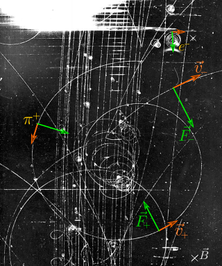
In physics, specifically in electromagnetism, the Lorentz force is the combination of electric and magnetic force on a point charge due to electromagnetic fields. A particle of charge q moving with a velocity v in an electric field E and a magnetic field B experiences a force of

<span class="mw-page-title-main">Work (physics)</span> Process of energy transfer to an object via force application through displacement

In physics, work is the energy transferred to or from an object via the application of force along a displacement. In its simplest form, for a constant force aligned with the direction of motion, the work equals the product of the force strength and the distance traveled. A force is said to do positive work if when applied it has a component in the direction of the displacement of the point of application. A force does negative work if it has a component opposite to the direction of the displacement at the point of application of the force.

<span class="mw-page-title-main">Fokker–Planck equation</span> Partial differential equation

In statistical mechanics and information theory, the Fokker–Planck equation is a partial differential equation that describes the time evolution of the probability density function of the velocity of a particle under the influence of drag forces and random forces, as in Brownian motion. The equation can be generalized to other observables as well. The Fokker-Planck equation has multiple applications in information theory, graph theory, data science, finance, economics etc.

In mathematics, differential forms provide a unified approach to define integrands over curves, surfaces, solids, and higher-dimensional manifolds. The modern notion of differential forms was pioneered by Élie Cartan. It has many applications, especially in geometry, topology and physics.

In vector calculus, Green's theorem relates a line integral around a simple closed curve C to a double integral over the plane region D bounded by C. It is the two-dimensional special case of Stokes' theorem.

In vector calculus, a conservative vector field is a vector field that is the gradient of some function. A conservative vector field has the property that its line integral is path independent; the choice of path between two points does not change the value of the line integral. Path independence of the line integral is equivalent to the vector field under the line integral being conservative. A conservative vector field is also irrotational; in three dimensions, this means that it has vanishing curl. An irrotational vector field is necessarily conservative provided that the domain is simply connected.

<span class="mw-page-title-main">Scalar potential</span> When potential energy difference depends only on displacement

In mathematical physics, scalar potential, simply stated, describes the situation where the difference in the potential energies of an object in two different positions depends only on the positions, not upon the path taken by the object in traveling from one position to the other. It is a scalar field in three-space: a directionless value (scalar) that depends only on its location. A familiar example is potential energy due to gravity.

In the mathematical field of complex analysis, contour integration is a method of evaluating certain integrals along paths in the complex plane.

In geometry and algebra, the triple product is a product of three 3-dimensional vectors, usually Euclidean vectors. The name "triple product" is used for two different products, the scalar-valued scalar triple product and, less often, the vector-valued vector triple product.

In calculus, the Leibniz integral rule for differentiation under the integral sign states that for an integral of the form

<span class="mw-page-title-main">Three-dimensional space</span> Geometric model of the physical space

In geometry, a three-dimensional space is a mathematical space in which three values (coordinates) are required to determine the position of a point. Most commonly, it is the three-dimensional Euclidean space, that is, the Euclidean space of dimension three, which models physical space. More general three-dimensional spaces are called 3-manifolds. The term may also refer colloquially to a subset of space, a three-dimensional region, a solid figure.

The following are important identities involving derivatives and integrals in vector calculus.

A parametric surface is a surface in the Euclidean space which is defined by a parametric equation with two parameters . Parametric representation is a very general way to specify a surface, as well as implicit representation. Surfaces that occur in two of the main theorems of vector calculus, Stokes' theorem and the divergence theorem, are frequently given in a parametric form. The curvature and arc length of curves on the surface, surface area, differential geometric invariants such as the first and second fundamental forms, Gaussian, mean, and principal curvatures can all be computed from a given parametrization.

A theoretical motivation for general relativity, including the motivation for the geodesic equation and the Einstein field equation, can be obtained from special relativity by examining the dynamics of particles in circular orbits about the Earth. A key advantage in examining circular orbits is that it is possible to know the solution of the Einstein Field Equation a priori. This provides a means to inform and verify the formalism.

<span class="mw-page-title-main">Covariant formulation of classical electromagnetism</span> Ways of writing certain laws of physics

The covariant formulation of classical electromagnetism refers to ways of writing the laws of classical electromagnetism in a form that is manifestly invariant under Lorentz transformations, in the formalism of special relativity using rectilinear inertial coordinate systems. These expressions both make it simple to prove that the laws of classical electromagnetism take the same form in any inertial coordinate system, and also provide a way to translate the fields and forces from one frame to another. However, this is not as general as Maxwell's equations in curved spacetime or non-rectilinear coordinate systems.

The gradient theorem, also known as the fundamental theorem of calculus for line integrals, says that a line integral through a gradient field can be evaluated by evaluating the original scalar field at the endpoints of the curve. The theorem is a generalization of the second fundamental theorem of calculus to any curve in a plane or space rather than just the real line.

<span class="mw-page-title-main">Differential geometry of surfaces</span> The mathematics of smooth surfaces

In mathematics, the differential geometry of surfaces deals with the differential geometry of smooth surfaces with various additional structures, most often, a Riemannian metric. Surfaces have been extensively studied from various perspectives: extrinsically, relating to their embedding in Euclidean space and intrinsically, reflecting their properties determined solely by the distance within the surface as measured along curves on the surface. One of the fundamental concepts investigated is the Gaussian curvature, first studied in depth by Carl Friedrich Gauss, who showed that curvature was an intrinsic property of a surface, independent of its isometric embedding in Euclidean space.

<span class="mw-page-title-main">Euclidean plane</span> Geometric model of the planar projection of the physical universe

In mathematics, a Euclidean plane is a Euclidean space of dimension two, denoted or . It is a geometric space in which two real numbers are required to determine the position of each point. It is an affine space, which includes in particular the concept of parallel lines. It has also metrical properties induced by a distance, which allows to define circles, and angle measurement.

<span class="mw-page-title-main">Stokes' theorem</span> Theorem in vector calculus

Stokes' theorem, also known as the Kelvin–Stokes theorem after Lord Kelvin and George Stokes, the fundamental theorem for curls or simply the curl theorem, is a theorem in vector calculus on . Given a vector field, the theorem relates the integral of the curl of the vector field over some surface, to the line integral of the vector field around the boundary of the surface. The classical theorem of Stokes can be stated in one sentence: The line integral of a vector field over a loop is equal to the surface integral of its curl over the enclosed surface. It is illustrated in the figure, where the direction of positive circulation of the bounding contour ∂Σ, and the direction n of positive flux through the surface Σ, are related by a right-hand-rule. For the right hand the fingers circulate along ∂Σ and the thumb is directed along n.

Lagrangian field theory is a formalism in classical field theory. It is the field-theoretic analogue of Lagrangian mechanics. Lagrangian mechanics is used to analyze the motion of a system of discrete particles each with a finite number of degrees of freedom. Lagrangian field theory applies to continua and fields, which have an infinite number of degrees of freedom.

References

  1. Kwong-Tin Tang (30 November 2006). Mathematical Methods for Engineers and Scientists 2: Vector Analysis, Ordinary Differential Equations and Laplace Transforms. Springer Science & Business Media. ISBN   978-3-540-30268-1.
  2. 1 2 Nykamp, Duane. "Line integrals are independent of parametrization". Math Insight. Retrieved September 18, 2020.
  3. "16.2 Line Integrals". www.whitman.edu. Retrieved 2020-09-18.
  4. Ahlfors, Lars (1966). Complex Analysis (2nd ed.). New York: McGraw-Hill. p. 103.