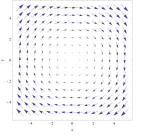
In vector calculus, the curl, also known as rotor, is a vector operator that describes the infinitesimal circulation of a vector field in three-dimensional Euclidean space. The curl at a point in the field is represented by a vector whose length and direction denote the magnitude and axis of the maximum circulation. The curl of a field is formally defined as the circulation density at each point of the field.
The derivative is a fundamental tool of calculus that quantifies the sensitivity of change of a function's output with respect to its input. The derivative of a function of a single variable at a chosen input value, when it exists, is the slope of the tangent line to the graph of the function at that point. The tangent line is the best linear approximation of the function near that input value. For this reason, the derivative is often described as the instantaneous rate of change, the ratio of the instantaneous change in the dependent variable to that of the independent variable. The process of finding a derivative is called differentiation.

In geometry, the tangent line (or simply tangent) to a plane curve at a given point is, intuitively, the straight line that "just touches" the curve at that point. Leibniz defined it as the line through a pair of infinitely close points on the curve. More precisely, a straight line is tangent to the curve y = f(x) at a point x = c if the line passes through the point (c, f(c)) on the curve and has slope f'(c), where f' is the derivative of f. A similar definition applies to space curves and curves in n-dimensional Euclidean space.
In mathematics, differential calculus is a subfield of calculus that studies the rates at which quantities change. It is one of the two traditional divisions of calculus, the other being integral calculus—the study of the area beneath a curve.
In mathematics, a partial derivative of a function of several variables is its derivative with respect to one of those variables, with the others held constant. Partial derivatives are used in vector calculus and differential geometry.

The Heaviside step function, or the unit step function, usually denoted by H or θ, is a step function named after Oliver Heaviside, the value of which is zero for negative arguments and one for nonnegative arguments. It is an example of the general class of step functions, all of which can be represented as linear combinations of translations of this one.

In probability theory and statistics, the beta distribution is a family of continuous probability distributions defined on the interval [0, 1] or in terms of two positive parameters, denoted by alpha (α) and beta (β), that appear as exponents of the variable and its complement to 1, respectively, and control the shape of the distribution.
On a differentiable manifold, the exterior derivative extends the concept of the differential of a function to differential forms of higher degree. The exterior derivative was first described in its current form by Élie Cartan in 1899. The resulting calculus, known as exterior calculus, allows for a natural, metric-independent generalization of Stokes' theorem, Gauss's theorem, and Green's theorem from vector calculus.
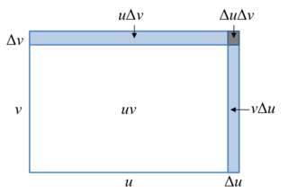
In calculus, the product rule is a formula used to find the derivatives of products of two or more functions. For two functions, it may be stated in Lagrange's notation as
In mathematics, the Gibbs phenomenon is the oscillatory behavior of the Fourier series of a piecewise continuously differentiable periodic function around a jump discontinuity. The th partial Fourier series of the function produces large peaks around the jump which overshoot and undershoot the function values. As more sinusoids are used, this approximation error approaches a limit of about 9% of the jump, though the infinite Fourier series sum does eventually converge almost everywhere except points of discontinuity.
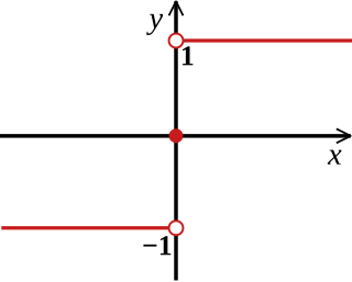
In mathematics, the sign function or signum function is a function that returns the sign of a real number. In mathematical notation the sign function is often represented as .
In multivariable calculus, the implicit function theorem is a tool that allows relations to be converted to functions of several real variables. It does so by representing the relation as the graph of a function. There may not be a single function whose graph can represent the entire relation, but there may be such a function on a restriction of the domain of the relation. The implicit function theorem gives a sufficient condition to ensure that there is such a function.
In mathematics, matrix calculus is a specialized notation for doing multivariable calculus, especially over spaces of matrices. It collects the various partial derivatives of a single function with respect to many variables, and/or of a multivariate function with respect to a single variable, into vectors and matrices that can be treated as single entities. This greatly simplifies operations such as finding the maximum or minimum of a multivariate function and solving systems of differential equations. The notation used here is commonly used in statistics and engineering, while the tensor index notation is preferred in physics.
In mathematics, the derivative is a fundamental construction of differential calculus and admits many possible generalizations within the fields of mathematical analysis, combinatorics, algebra, geometry, etc.
In mathematics, the symmetric derivative is an operation generalizing the ordinary derivative.
In differential calculus, there is no single uniform notation for differentiation. Instead, various notations for the derivative of a function or variable have been proposed by various mathematicians. The usefulness of each notation varies with the context, and it is sometimes advantageous to use more than one notation in a given context. The most common notations for differentiation are listed below.
This is a summary of differentiation rules, that is, rules for computing the derivative of a function in calculus.

The differentiation of trigonometric functions is the mathematical process of finding the derivative of a trigonometric function, or its rate of change with respect to a variable. For example, the derivative of the sine function is written sin′(a) = cos(a), meaning that the rate of change of sin(x) at a particular angle x = a is given by the cosine of that angle.
Most of the terms listed in Wikipedia glossaries are already defined and explained within Wikipedia itself. However, glossaries like this one are useful for looking up, comparing and reviewing large numbers of terms together. You can help enhance this page by adding new terms or writing definitions for existing ones.
In mathematics, calculus on Euclidean space is a generalization of calculus of functions in one or several variables to calculus of functions on Euclidean space as well as a finite-dimensional real vector space. This calculus is also known as advanced calculus, especially in the United States. It is similar to multivariable calculus but is somewhat more sophisticated in that it uses linear algebra more extensively and covers some concepts from differential geometry such as differential forms and Stokes' formula in terms of differential forms. This extensive use of linear algebra also allows a natural generalization of multivariable calculus to calculus on Banach spaces or topological vector spaces.


![A plot of
f
(
x
)
=
sin
[?]
(
2
x
)
{\displaystyle f(x)=\sin(2x)}
from
-
p
/
4
{\displaystyle -\pi /4}
to
5
p
/
4
{\displaystyle 5\pi /4}
. The tangent line is blue where the curve is concave up, green where the curve is concave down, and red at the inflection points (0,
p
{\displaystyle \pi }
/2, and
p
{\displaystyle \pi }
). Animated illustration of inflection point.gif](http://upload.wikimedia.org/wikipedia/commons/7/78/Animated_illustration_of_inflection_point.gif)


