The partial derivative of a function with respect to the variable is variously denoted by
, , , , , , or .
It can be thought of as the rate of change of the function in the -direction.
Sometimes, for , the partial derivative of with respect to is denoted as Since a partial derivative generally has the same arguments as the original function, its functional dependence is sometimes explicitly signified by the notation, such as in:
The symbol used to denote partial derivatives is ∂. One of the first known uses of this symbol in mathematics is by Marquis de Condorcet from 1770,[1] who used it for partial differences. The modern partial derivative notation was created by Adrien-Marie Legendre (1786), although he later abandoned it; Carl Gustav Jacob Jacobi reintroduced the symbol in 1841.[2]
Definition
Like ordinary derivatives, the partial derivative is defined as a limit. Let U be an open subset of and a function. The partial derivative of f at the point with respect to the i-th variable xi is defined as
Where is the unit vector of i-th variable xi. Even if all partial derivatives exist at a given point a, the function need not be continuous there. However, if all partial derivatives exist in a neighborhood of a and are continuous there, then f is totally differentiable in that neighborhood and the total derivative is continuous. In this case, it is said that f is a C1 function. This can be used to generalize for vector valued functions, , by carefully using a componentwise argument.
The partial derivative can be seen as another function defined on U and can again be partially differentiated. If the direction of derivative is not repeated, it is called a mixed partial derivative. If all mixed second order partial derivatives are continuous at a point (or on a set), f is termed a C2 function at that point (or on that set); in this case, the partial derivatives can be exchanged by Clairaut's theorem:
When dealing with functions of multiple variables, some of these variables may be related to each other, thus it may be necessary to specify explicitly which variables are being held constant to avoid ambiguity. In fields such as statistical mechanics, the partial derivative of f with respect to x, holding y and z constant, is often expressed as
Conventionally, for clarity and simplicity of notation, the partial derivative function and the value of the function at a specific point are conflated by including the function arguments when the partial derivative symbol (Leibniz notation) is used. Thus, an expression like
is used for the function, while
might be used for the value of the function at the point . However, this convention breaks down when we want to evaluate the partial derivative at a point like . In such a case, evaluation of the function must be expressed in an unwieldy manner as
or
in order to use the Leibniz notation. Thus, in these cases, it may be preferable to use the Euler differential operator notation with as the partial derivative symbol with respect to the i-th variable. For instance, one would write for the example described above, while the expression represents the partial derivative function with respect to the first variable.[3]
For higher order partial derivatives, the partial derivative (function) of with respect to the j-th variable is denoted . That is, , so that the variables are listed in the order in which the derivatives are taken, and thus, in reverse order of how the composition of operators is usually notated. Of course, Clairaut's theorem implies that as long as comparatively mild regularity conditions on f are satisfied.
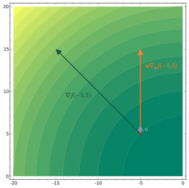
An important example of a function of several variables is the case of a scalar-valued function on a domain in Euclidean space (e.g., on or ). In this case f has a partial derivative with respect to each variable xj. At the point a, these partial derivatives define the vector
This vector is called the gradient of f at a. If f is differentiable at every point in some domain, then the gradient is a vector-valued function ∇f which takes the point a to the vector ∇f(a). Consequently, the gradient produces a vector field.
A contour plot of , showing the gradient vector in black, and the unit vector scaled by the directional derivative in the direction of in orange. The gradient vector is longer because the gradient points in the direction of greatest rate of increase of a function.
This definition is valid in a broad range of contexts, for example where the norm of a vector (and hence a unit vector) is undefined.[5]
Example
Suppose that f is a function of more than one variable. For instance,
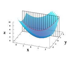
A graph of z = x2 + xy + y2. For the partial derivative at (1, 1) that leaves y constant, the corresponding tangent line is parallel to the xz-plane.
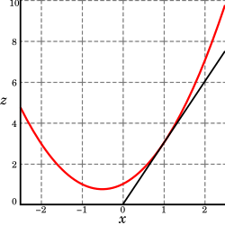
A slice of the graph above showing the function in the xz-plane at y = 1. Note that the two axes are shown here with different scales. The slope of the tangent line is 3.
The graph of this function defines a surface in Euclidean space. To every point on this surface, there are an infinite number of tangent lines. Partial differentiation is the act of choosing one of these lines and finding its slope. Usually, the lines of most interest are those that are parallel to the xz-plane, and those that are parallel to the yz-plane (which result from holding either y or x constant, respectively).
To find the slope of the line tangent to the function at P(1, 1) and parallel to the xz-plane, we treat y as a constant. The graph and this plane are shown on the right. Below, we see how the function looks on the plane y = 1. By finding the derivative of the equation while assuming that y is a constant, we find that the slope of f at the point (x, y) is:
So at (1, 1), by substitution, the slope is 3. Therefore,
at the point (1, 1). That is, the partial derivative of z with respect to x at (1, 1) is 3, as shown in the graph.
The function f can be reinterpreted as a family of functions of one variable indexed by the other variables:
In other words, every value of y defines a function, denoted fy, which is a function of one variable x.[6] That is,
In this section the subscript notation fy denotes a function contingent on a fixed value of y, and not a partial derivative.
Once a value of y is chosen, say a, then f(x,y) determines a function fa which traces a curve x2 + ax + a2 on the xz-plane:
In this expression, a is a constant, not a variable, so fa is a function of only one real variable, that being x. Consequently, the definition of the derivative for a function of one variable applies:
The above procedure can be performed for any choice of a. Assembling the derivatives together into a function gives a function which describes the variation of f in the x direction:
This is the partial derivative of f with respect to x. Here '∂' is a rounded 'd' called the partial derivative symbol; to distinguish it from the letter 'd', '∂' is sometimes pronounced "partial".
Higher order partial derivatives
Second and higher order partial derivatives are defined analogously to the higher order derivatives of univariate functions. For the function the "own" second partial derivative with respect to x is simply the partial derivative of the partial derivative (both with respect to x):[7]:316–318
The cross partial derivative with respect to x and y is obtained by taking the partial derivative of f with respect to x, and then taking the partial derivative of the result with respect to y, to obtain
Schwarz's theorem states that if the second derivatives are continuous, the expression for the cross partial derivative is unaffected by which variable the partial derivative is taken with respect to first and which is taken second. That is,
or equivalently
Own and cross partial derivatives appear in the Hessian matrix which is used in the second order conditions in optimization problems. The higher order partial derivatives can be obtained by successive differentiation
Antiderivative analogue
There is a concept for partial derivatives that is analogous to antiderivatives for regular derivatives. Given a partial derivative, it allows for the partial recovery of the original function.
Consider the example of
The so-called partial integral can be taken with respect to x (treating y as constant, in a similar manner to partial differentiation):
Here, the constant of integration is no longer a constant, but instead a function of all the variables of the original function except x. The reason for this is that all the other variables are treated as constant when taking the partial derivative, so any function which does not involve x will disappear when taking the partial derivative, and we have to account for this when we take the antiderivative. The most general way to represent this is to have the constant represent an unknown function of all the other variables.
Thus the set of functions , where g is any one-argument function, represents the entire set of functions in variables x, y that could have produced the x-partial derivative .
If all the partial derivatives of a function are known (for example, with the gradient), then the antiderivatives can be matched via the above process to reconstruct the original function up to a constant. Unlike in the single-variable case, however, not every set of functions can be the set of all (first) partial derivatives of a single function. In other words, not every vector field is conservative.
Applications
Geometry
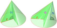
The volume of a cone depends on height and radius
The volumeV of a cone depends on the cone's heighth and its radiusr according to the formula
The partial derivative of V with respect to r is
which represents the rate with which a cone's volume changes if its radius is varied and its height is kept constant. The partial derivative with respect to h equals , which represents the rate with which the volume changes if its height is varied and its radius is kept constant.
By contrast, the total derivative of V with respect to r and h are respectively
The difference between the total and partial derivative is the elimination of indirect dependencies between variables in partial derivatives.
If (for some arbitrary reason) the cone's proportions have to stay the same, and the height and radius are in a fixed ratio k,
This gives the total derivative with respect to r,
which simplifies to
Similarly, the total derivative with respect to h is
The total derivative with respect to bothr and h of the volume intended as scalar function of these two variables is given by the gradient vector
Optimization
Partial derivatives appear in any calculus-based optimization problem with more than one choice variable. For example, in economics a firm may wish to maximize profitπ(x, y) with respect to the choice of the quantities x and y of two different types of output. The first order conditions for this optimization are πx = 0 = πy. Since both partial derivatives πx and πy will generally themselves be functions of both arguments x and y, these two first order conditions form a system of two equations in two unknowns.
Thermodynamics, quantum mechanics and mathematical physics
Partial derivatives appear in thermodynamic equations like Gibbs-Duhem equation, in quantum mechanics as Schrodinger wave equation as well in other equations from mathematical physics. Here the variables being held constant in partial derivatives can be ratio of simple variables like mole fractionsxi in the following example involving the Gibbs energies in a ternary mixture system:
Express mole fractions of a component as functions of other components' mole fraction and binary mole ratios:
Differential quotients can be formed at constant ratios like those above:
Ratios X, Y, Z of mole fractions can be written for ternary and multicomponent systems:
This equality can be rearranged to have differential quotient of mole fractions on one side.
Image resizing
Partial derivatives are key to target-aware image resizing algorithms. Widely known as seam carving, these algorithms require each pixel in an image to be assigned a numerical 'energy' to describe their dissimilarity against orthogonal adjacent pixels. The algorithm then progressively removes rows or columns with the lowest energy. The formula established to determine a pixel's energy (magnitude of gradient at a pixel) depends heavily on the constructs of partial derivatives.
Economics
Partial derivatives play a prominent role in economics, in which most functions describing economic behaviour posit that the behaviour depends on more than one variable. For example, a societal consumption function may describe the amount spent on consumer goods as depending on both income and wealth; the marginal propensity to consume is then the partial derivative of the consumption function with respect to income.
In calculus, the chain rule is a formula that expresses the derivative of the composition of two differentiable functions f and g in terms of the derivatives of f and g. More precisely, if is the function such that for every x, then the chain rule is, in Lagrange's notation,
The derivative is a fundamental tool of calculus that quantifies the sensitivity of change of a function's output with respect to its input. The derivative of a function of a single variable at a chosen input value, when it exists, is the slope of the tangent line to the graph of the function at that point. The tangent line is the best linear approximation of the function near that input value. For this reason, the derivative is often described as the instantaneous rate of change, the ratio of the instantaneous change in the dependent variable to that of the independent variable. The process of finding a derivative is called differentiation.
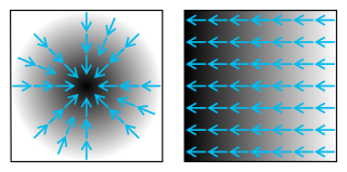
In vector calculus, divergence is a vector operator that operates on a vector field, producing a scalar field giving the quantity of the vector field's source at each point. More technically, the divergence represents the volume density of the outward flux of a vector field from an infinitesimal volume around a given point.
In vector calculus, the gradient of a scalar-valued differentiable function of several variables is the vector field whose value at a point gives the direction and the rate of fastest increase. The gradient transforms like a vector under change of basis of the space of variables of . If the gradient of a function is non-zero at a point , the direction of the gradient is the direction in which the function increases most quickly from , and the magnitude of the gradient is the rate of increase in that direction, the greatest absolute directional derivative. Further, a point where the gradient is the zero vector is known as a stationary point. The gradient thus plays a fundamental role in optimization theory, where it is used to minimize a function by gradient descent. In coordinate-free terms, the gradient of a function may be defined by:
In probability theory, a probability density function (PDF), density function, or density of an absolutely continuous random variable, is a function whose value at any given sample in the sample space can be interpreted as providing a relative likelihood that the value of the random variable would be equal to that sample. Probability density is the probability per unit length, in other words, while the absolute likelihood for a continuous random variable to take on any particular value is 0, the value of the PDF at two different samples can be used to infer, in any particular draw of the random variable, how much more likely it is that the random variable would be close to one sample compared to the other sample.
The Navier–Stokes equations are partial differential equations which describe the motion of viscous fluid substances. They were named after French engineer and physicist Claude-Louis Navier and the Irish physicist and mathematician George Gabriel Stokes. They were developed over several decades of progressively building the theories, from 1822 (Navier) to 1842–1850 (Stokes).
A Fourier series is an expansion of a periodic function into a sum of trigonometric functions. The Fourier series is an example of a trigonometric series, but not all trigonometric series are Fourier series. By expressing a function as a sum of sines and cosines, many problems involving the function become easier to analyze because trigonometric functions are well understood. For example, Fourier series were first used by Joseph Fourier to find solutions to the heat equation. This application is possible because the derivatives of trigonometric functions fall into simple patterns. Fourier series cannot be used to approximate arbitrary functions, because most functions have infinitely many terms in their Fourier series, and the series do not always converge. Well-behaved functions, for example smooth functions, have Fourier series that converge to the original function. The coefficients of the Fourier series are determined by integrals of the function multiplied by trigonometric functions, described in Common forms of the Fourier series below.
In mathematics, Cauchy's integral formula, named after Augustin-Louis Cauchy, is a central statement in complex analysis. It expresses the fact that a holomorphic function defined on a disk is completely determined by its values on the boundary of the disk, and it provides integral formulas for all derivatives of a holomorphic function. Cauchy's formula shows that, in complex analysis, "differentiation is equivalent to integration": complex differentiation, like integration, behaves well under uniform limits – a result that does not hold in real analysis.
A mathematical symbol is a figure or a combination of figures that is used to represent a mathematical object, an action on mathematical objects, a relation between mathematical objects, or for structuring the other symbols that occur in a formula. As formulas are entirely constituted with symbols of various types, many symbols are needed for expressing all mathematics.
In vector calculus, the Jacobian matrix of a vector-valued function of several variables is the matrix of all its first-order partial derivatives. When this matrix is square, that is, when the function takes the same number of variables as input as the number of vector components of its output, its determinant is referred to as the Jacobian determinant. Both the matrix and the determinant are often referred to simply as the Jacobian in literature.
In vector calculus, Green's theorem relates a line integral around a simple closed curve C to a double integral over the plane region D bounded by C. It is the two-dimensional special case of Stokes' theorem.
In probability and statistics, an exponential family is a parametric set of probability distributions of a certain form, specified below. This special form is chosen for mathematical convenience, including the enabling of the user to calculate expectations, covariances using differentiation based on some useful algebraic properties, as well as for generality, as exponential families are in a sense very natural sets of distributions to consider. The term exponential class is sometimes used in place of "exponential family", or the older term Koopman–Darmois family. Sometimes loosely referred to as "the" exponential family, this class of distributions is distinct because they all possess a variety of desirable properties, most importantly the existence of a sufficient statistic.
In mathematics, the Hessian matrix, Hessian or Hesse matrix is a square matrix of second-order partial derivatives of a scalar-valued function, or scalar field. It describes the local curvature of a function of many variables. The Hessian matrix was developed in the 19th century by the German mathematician Ludwig Otto Hesse and later named after him. Hesse originally used the term "functional determinants". The Hessian is sometimes denoted by H or, ambiguously, by ∇2.
In mathematics, the covariant derivative is a way of specifying a derivative along tangent vectors of a manifold. Alternatively, the covariant derivative is a way of introducing and working with a connection on a manifold by means of a differential operator, to be contrasted with the approach given by a principal connection on the frame bundle – see affine connection. In the special case of a manifold isometrically embedded into a higher-dimensional Euclidean space, the covariant derivative can be viewed as the orthogonal projection of the Euclidean directional derivative onto the manifold's tangent space. In this case the Euclidean derivative is broken into two parts, the extrinsic normal component and the intrinsic covariant derivative component.
In multivariable calculus, the implicit function theorem is a tool that allows relations to be converted to functions of several real variables. It does so by representing the relation as the graph of a function. There may not be a single function whose graph can represent the entire relation, but there may be such a function on a restriction of the domain of the relation. The implicit function theorem gives a sufficient condition to ensure that there is such a function.
The following are important identities involving derivatives and integrals in vector calculus.
A vector-valued function, also referred to as a vector function, is a mathematical function of one or more variables whose range is a set of multidimensional vectors or infinite-dimensional vectors. The input of a vector-valued function could be a scalar or a vector ; the dimension of the function's domain has no relation to the dimension of its range.
In differential calculus, there is no single uniform notation for differentiation. Instead, various notations for the derivative of a function or variable have been proposed by various mathematicians. The usefulness of each notation varies with the context, and it is sometimes advantageous to use more than one notation in a given context. The most common notations for differentiation are listed below.
In mathematical analysis and its applications, a function of several real variables or real multivariate function is a function with more than one argument, with all arguments being real variables. This concept extends the idea of a function of a real variable to several variables. The "input" variables take real values, while the "output", also called the "value of the function", may be real or complex. However, the study of the complex-valued functions may be easily reduced to the study of the real-valued functions, by considering the real and imaginary parts of the complex function; therefore, unless explicitly specified, only real-valued functions will be considered in this article.
In theoretical physics, Hamiltonian field theory is the field-theoretic analogue to classical Hamiltonian mechanics. It is a formalism in classical field theory alongside Lagrangian field theory. It also has applications in quantum field theory.
This page is based on this Wikipedia article Text is available under the CC BY-SA 4.0 license; additional terms may apply. Images, videos and audio are available under their respective licenses.