Integration by substitution

Last updated

In calculus, integration by substitution, also known as u-substitution, reverse chain rule or change of variables, [1] is a method for evaluating integrals and antiderivatives. It is the counterpart to the chain rule for differentiation, and can loosely be thought of as using the chain rule "backwards."

Contents

Substitution for a single variable

Introduction (indefinite integrals)

Before stating the result rigorously, consider a simple case using indefinite integrals.

Compute [2]

Set This means or as a differential form, Now:

where is an arbitrary constant of integration.

This procedure is frequently used, but not all integrals are of a form that permits its use. In any event, the result should be verified by differentiating and comparing to the original integrand.

For definite integrals, the limits of integration must also be adjusted, but the procedure is mostly the same.

Statement for definite integrals

Let be a differentiable function with a continuous derivative, where is an interval. Suppose that is a continuous function. Then: [3]

In Leibniz notation, the substitution yields:

Working heuristically with infinitesimals yields the equation

which suggests the substitution formula above. (This equation may be put on a rigorous foundation by interpreting it as a statement about differential forms.) One may view the method of integration by substitution as a partial justification of Leibniz's notation for integrals and derivatives.

The formula is used to transform one integral into another integral that is easier to compute. Thus, the formula can be read from left to right or from right to left in order to simplify a given integral. When used in the former manner, it is sometimes known as u-substitution or w-substitution in which a new variable is defined to be a function of the original variable found inside the composite function multiplied by the derivative of the inner function. The latter manner is commonly used in trigonometric substitution, replacing the original variable with a trigonometric function of a new variable and the original differential with the differential of the trigonometric function.

Proof

Integration by substitution can be derived from the fundamental theorem of calculus as follows. Let and be two functions satisfying the above hypothesis that is continuous on and is integrable on the closed interval . Then the function is also integrable on . Hence the integrals

and

in fact exist, and it remains to show that they are equal.

Since is continuous, it has an antiderivative . The composite function is then defined. Since is differentiable, combining the chain rule and the definition of an antiderivative gives:

Applying the fundamental theorem of calculus twice gives:

which is the substitution rule.

Examples: Definite integrals

Example 1

Consider the integral:

Make the substitution to obtain meaning Therefore:

Since the lower limit was replaced with and the upper limit with a transformation back into terms of was unnecessary.

Alternatively, one may fully evaluate the indefinite integral (see below) first then apply the boundary conditions. This becomes especially handy when multiple substitutions are used.

Example 2

For the integral

a variation of the above procedure is needed. The substitution implying is useful because We thus have:

The resulting integral can be computed using integration by parts or a double angle formula, followed by one more substitution. One can also note that the function being integrated is the upper right quarter of a circle with a radius of one, and hence integrating the upper right quarter from zero to one is the geometric equivalent to the area of one quarter of the unit circle, or

Examples: Antiderivatives

Substitution can be used to determine antiderivatives. One chooses a relation between and determines the corresponding relation between and by differentiating, and performs the substitutions. An antiderivative for the substituted function can hopefully be determined; the original substitution between and is then undone.

Similar to example 1 above, the following antiderivative can be obtained with this method:

where is an arbitrary constant of integration.

There were no integral boundaries to transform, but in the last step reverting the original substitution was necessary. When evaluating definite integrals by substitution, one may calculate the antiderivative fully first, then apply the boundary conditions. In that case, there is no need to transform the boundary terms.

Trigonometric functions

The tangent function can be integrated using substitution by expressing it in terms of the sine and cosine: .

Using the substitution gives and

The cotangent function can be integrated similarly by expressing it as and using the substitution :

Substitution for multiple variables

One may also use substitution when integrating functions of several variables.

Here, the substitution function (v1,...,vn) = φ(u1, ..., un) needs to be injective and continuously differentiable, and the differentials transform as:

where det()(u1, ..., un) denotes the determinant of the Jacobian matrix of partial derivatives of φ at the point (u1, ..., un). This formula expresses the fact that the absolute value of the determinant of a matrix equals the volume of the parallelotope spanned by its columns or rows.

More precisely, the change of variables formula is stated in the next theorem:

Theorem  Let U be an open set in Rn and φ : URn an injective differentiable function with continuous partial derivatives, the Jacobian of which is nonzero for every x in U. Then for any real-valued, compactly supported, continuous function f, with support contained in φ(U):

The conditions on the theorem can be weakened in various ways. First, the requirement that φ be continuously differentiable can be replaced by the weaker assumption that φ be merely differentiable and have a continuous inverse. [4] This is guaranteed to hold if φ is continuously differentiable by the inverse function theorem. Alternatively, the requirement that det() ≠ 0 can be eliminated by applying Sard's theorem. [5]

For Lebesgue measurable functions, the theorem can be stated in the following form: [6]

Theorem  Let U be a measurable subset of Rn and φ : URn an injective function, and suppose for every x in U there exists φ(x) in Rn,n such that φ(y) = φ(x) + φ(x)(yx) + o(yx) as yx (here o is little-o notation). Then φ(U) is measurable, and for any real-valued function f defined on φ(U):

in the sense that if either integral exists (including the possibility of being properly infinite), then so does the other one, and they have the same value.

Another very general version in measure theory is the following: [7]

Theorem  Let X be a locally compact Hausdorff space equipped with a finite Radon measure μ, and let Y be a σ-compact Hausdorff space with a σ-finite Radon measure ρ. Let φ : XY be an absolutely continuous function (where the latter means that ρ(φ(E)) = 0 whenever μ(E) = 0). Then there exists a real-valued Borel measurable function w on X such that for every Lebesgue integrable function f : YR, the function (fφ) ⋅ w is Lebesgue integrable on X, and

Furthermore, it is possible to write

for some Borel measurable function g on Y.

In geometric measure theory, integration by substitution is used with Lipschitz functions. A bi-Lipschitz function is a Lipschitz function φ : URn which is injective and whose inverse function φ1 : φ(U) → U is also Lipschitz. By Rademacher's theorem, a bi-Lipschitz mapping is differentiable almost everywhere. In particular, the Jacobian determinant of a bi-Lipschitz mapping det is well-defined almost everywhere. The following result then holds:

Theorem  Let U be an open subset of Rn and φ : URn be a bi-Lipschitz mapping. Let f : φ(U) → R be measurable. Then

in the sense that if either integral exists (or is properly infinite), then so does the other one, and they have the same value.

The above theorem was first proposed by Euler when he developed the notion of double integrals in 1769. Although generalized to triple integrals by Lagrange in 1773, and used by Legendre, Laplace, and Gauss, and first generalized to n variables by Mikhail Ostrogradsky in 1836, it resisted a fully rigorous formal proof for a surprisingly long time, and was first satisfactorily resolved 125 years later, by Élie Cartan in a series of papers beginning in the mid-1890s. [8] [9]

Application in probability

Substitution can be used to answer the following important question in probability: given a random variable X with probability density pX and another random variable Y such that Y= ϕ(X) for injective (one-to-one) ϕ, what is the probability density for Y?

It is easiest to answer this question by first answering a slightly different question: what is the probability that Y takes a value in some particular subset S? Denote this probability P(YS). Of course, if Y has probability density pY, then the answer is:

but this is not really useful because we do not know pY; it is what we are trying to find. We can make progress by considering the problem in the variable X. Y takes a value in S whenever X takes a value in so:

Changing from variable x to y gives:

Combining this with our first equation gives:

so:

In the case where X and Y depend on several uncorrelated variables (i.e., and ), can be found by substitution in several variables discussed above. The result is:

See also

Notes

  1. Swokowski 1983 , p. 257
  2. Swokowski 1983 , p. 258
  3. Briggs & Cochran 2011 , p. 361
  4. Rudin 1987 , Theorem 7.26
  5. Spivak 1965 , p. 72
  6. Fremlin 2010 , Theorem 263D
  7. Hewitt & Stromberg 1965 , Theorem 20.3
  8. Katz 1982
  9. Ferzola 1994

Related Research Articles

<span class="mw-page-title-main">Euler's formula</span> Complex exponential in terms of sine and cosine

Euler's formula, named after Leonhard Euler, is a mathematical formula in complex analysis that establishes the fundamental relationship between the trigonometric functions and the complex exponential function. Euler's formula states that, for any real number x, one has

In mathematics, the Laplace transform, named after its discoverer Pierre-Simon Laplace, is an integral transform that converts a function of a real variable to a function of a complex variable .

<span class="mw-page-title-main">Mean value theorem</span> On the existence of a tangent to an arc parallel to the line through its endpoints

In mathematics, the mean value theorem states, roughly, that for a given planar arc between two endpoints, there is at least one point at which the tangent to the arc is parallel to the secant through its endpoints. It is one of the most important results in real analysis. This theorem is used to prove statements about a function on an interval starting from local hypotheses about derivatives at points of the interval.

<span class="mw-page-title-main">Polar coordinate system</span> Coordinates comprising a distance and an angle

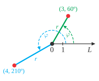
In mathematics, the polar coordinate system is a two-dimensional coordinate system in which each point on a plane is determined by a distance from a reference point and an angle from a reference direction. The reference point is called the pole, and the ray from the pole in the reference direction is the polar axis. The distance from the pole is called the radial coordinate, radial distance or simply radius, and the angle is called the angular coordinate, polar angle, or azimuth. Angles in polar notation are generally expressed in either degrees or radians.

<span class="mw-page-title-main">Laplace's equation</span> Second-order partial differential equation

In mathematics and physics, Laplace's equation is a second-order partial differential equation named after Pierre-Simon Laplace, who first studied its properties. This is often written as

<span class="mw-page-title-main">Dirac delta function</span> Generalized function whose value is zero everywhere except at zero

In mathematical analysis, the Dirac delta function, also known as the unit impulse, is a generalized function on the real numbers, whose value is zero everywhere except at zero, and whose integral over the entire real line is equal to one. Since there is no function having this property, to model the delta "function" rigorously involves the use of limits or, as is common in mathematics, measure theory and the theory of distributions.

<span class="mw-page-title-main">Fourier series</span> Decomposition of periodic functions into sums of simpler sinusoidal forms

A Fourier series is an expansion of a periodic function into a sum of trigonometric functions. The Fourier series is an example of a trigonometric series, but not all trigonometric series are Fourier series. By expressing a function as a sum of sines and cosines, many problems involving the function become easier to analyze because trigonometric functions are well understood. For example, Fourier series were first used by Joseph Fourier to find solutions to the heat equation. This application is possible because the derivatives of trigonometric functions fall into simple patterns. Fourier series cannot be used to approximate arbitrary functions, because most functions have infinitely many terms in their Fourier series, and the series do not always converge. Well-behaved functions, for example smooth functions, have Fourier series that converge to the original function. The coefficients of the Fourier series are determined by integrals of the function multiplied by trigonometric functions, described in Common forms of the Fourier series below.

In calculus, and more generally in mathematical analysis, integration by parts or partial integration is a process that finds the integral of a product of functions in terms of the integral of the product of their derivative and antiderivative. It is frequently used to transform the antiderivative of a product of functions into an antiderivative for which a solution can be more easily found. The rule can be thought of as an integral version of the product rule of differentiation; it is indeed derived using the product rule.

In vector calculus, the Jacobian matrix of a vector-valued function of several variables is the matrix of all its first-order partial derivatives. When this matrix is square, that is, when the function takes the same number of variables as input as the number of vector components of its output, its determinant is referred to as the Jacobian determinant. Both the matrix and the determinant are often referred to simply as the Jacobian in literature.

<span class="mw-page-title-main">Green's function</span> Impulse response of an inhomogeneous linear differential operator

In mathematics, a Green's function is the impulse response of an inhomogeneous linear differential operator defined on a domain with specified initial conditions or boundary conditions.

In mathematics, the Mellin transform is an integral transform that may be regarded as the multiplicative version of the two-sided Laplace transform. This integral transform is closely connected to the theory of Dirichlet series, and is often used in number theory, mathematical statistics, and the theory of asymptotic expansions; it is closely related to the Laplace transform and the Fourier transform, and the theory of the gamma function and allied special functions.

<span class="mw-page-title-main">Path integral formulation</span> Formulation of quantum mechanics

The path integral formulation is a description in quantum mechanics that generalizes the stationary action principle of classical mechanics. It replaces the classical notion of a single, unique classical trajectory for a system with a sum, or functional integral, over an infinity of quantum-mechanically possible trajectories to compute a quantum amplitude.

<span class="mw-page-title-main">Stable distribution</span> Distribution of variables which satisfies a stability property under linear combinations

In probability theory, a distribution is said to be stable if a linear combination of two independent random variables with this distribution has the same distribution, up to location and scale parameters. A random variable is said to be stable if its distribution is stable. The stable distribution family is also sometimes referred to as the Lévy alpha-stable distribution, after Paul Lévy, the first mathematician to have studied it.

In mathematics, a change of variables is a basic technique used to simplify problems in which the original variables are replaced with functions of other variables. The intent is that when expressed in new variables, the problem may become simpler, or equivalent to a better understood problem.

In calculus, the Leibniz integral rule for differentiation under the integral sign states that for an integral of the form

<span class="mw-page-title-main">Multiple integral</span> Generalization of definite integrals to functions of multiple variables

In mathematics (specifically multivariable calculus), a multiple integral is a definite integral of a function of several real variables, for instance, f(x, y) or f(x, y, z). Physical (natural philosophy) interpretation: S any surface, V any volume, etc.. Incl. variable to time, position, etc.

Common integrals in quantum field theory are all variations and generalizations of Gaussian integrals to the complex plane and to multiple dimensions. Other integrals can be approximated by versions of the Gaussian integral. Fourier integrals are also considered.

In integral calculus, the tangent half-angle substitution is a change of variables used for evaluating integrals, which converts a rational function of trigonometric functions of into an ordinary rational function of by setting . This is the one-dimensional stereographic projection of the unit circle parametrized by angle measure onto the real line. The general transformation formula is:

<span class="mw-page-title-main">Integral of the secant function</span> Antiderivative of the secant function

In calculus, the integral of the secant function can be evaluated using a variety of methods and there are multiple ways of expressing the antiderivative, all of which can be shown to be equivalent via trigonometric identities,

In mathematics, calculus on Euclidean space is a generalization of calculus of functions in one or several variables to calculus of functions on Euclidean space as well as a finite-dimensional real vector space. This calculus is also known as advanced calculus, especially in the United States. It is similar to multivariable calculus but is somewhat more sophisticated in that it uses linear algebra more extensively and covers some concepts from differential geometry such as differential forms and Stokes' formula in terms of differential forms. This extensive use of linear algebra also allows a natural generalization of multivariable calculus to calculus on Banach spaces or topological vector spaces.

References