Loop-erased random walk

Last updated
A loop-erased random walk in 2D for
10
6
{\displaystyle 10^{6}}
steps. Loop erased random walk in 2D.png
A loop-erased random walk in 2D for steps.

In mathematics, loop-erased random walk is a model for a random simple path with important applications in combinatorics, physics and quantum field theory. It is intimately connected to the uniform spanning tree, a model for a random tree. See also random walk for more general treatment of this topic.

Contents

Definition

Assume G is some graph and is some path of length n on G. In other words, are vertices of G such that and are connected by an edge. Then the loop erasure of is a new simple path created by erasing all the loops of in chronological order. Formally, we define indices inductively using

where "max" here means up to the length of the path . The induction stops when for some we have .

In words, to find , we hold in one hand, and with the other hand, we trace back from the end: , until we either hit some , in which case we set , or we end up at , in which case we set .

Assume this happens at J i.e. is the last . Then the loop erasure of , denoted by is a simple path of length J defined by

Now let G be some graph, let v be a vertex of G, and let R be a random walk on G starting from v. Let T be some stopping time for R. Then the loop-erased random walk until time T is LE(R([1,T])). In other words, take R from its beginning until T — that's a (random) path — erase all the loops in chronological order as above — you get a random simple path.

The stopping time T may be fixed, i.e. one may perform n steps and then loop-erase. However, it is usually more natural to take T to be the hitting time in some set. For example, let G be the graph Z2 and let R be a random walk starting from the point (0,0). Let T be the time when R first hits the circle of radius 100 (we mean here of course a discretized circle). LE(R) is called the loop-erased random walk starting at (0,0) and stopped at the circle.

Uniform spanning tree

For any graph G, a spanning tree of G is a subgraph of G containing all vertices and some of the edges, which is a tree, i.e. connected and with no cycles. A spanning tree chosen randomly from among all possible spanning trees with equal probability is called a uniform spanning tree. There are typically exponentially many spanning trees (too many to generate them all and then choose one randomly); instead, uniform spanning trees can be generated more efficiently by an algorithm called Wilson's algorithm which uses loop-erased random walks.

The algorithm proceeds according to the following steps. First, construct a single-vertex tree T by choosing (arbitrarily) one vertex. Then, while the tree T constructed so far does not yet include all of the vertices of the graph, let v be an arbitrary vertex that is not in T, perform a loop-erased random walk from v until reaching a vertex in T, and add the resulting path to T. Repeating this process until all vertices are included produces a uniformly distributed tree, regardless of the arbitrary choices of vertices at each step.

A connection in the other direction is also true. If v and w are two vertices in G then, in any spanning tree, they are connected by a unique path. Taking this path in the uniform spanning tree gives a random simple path. It turns out that the distribution of this path is identical to the distribution of the loop-erased random walk starting at v and stopped at w. This fact can be used to justify the correctness of Wilson's algorithm. Another corollary is that loop-erased random walk is symmetric in its start and end points. More precisely, the distribution of the loop-erased random walk starting at v and stopped at w is identical to the distribution of the reversal of loop-erased random walk starting at w and stopped at v. Loop-erasing a random walk and the reverse walk do not, in general, give the same result, but according to this result the distributions of the two loop-erased walks are identical.

The Laplacian random walk

Another representation of loop-erased random walk stems from solutions of the discrete Laplace equation. Let G again be a graph and let v and w be two vertices in G. Construct a random path from v to w inductively using the following procedure. Assume we have already defined . Let f be a function from G to R satisfying

for all and
f is discretely harmonic everywhere else

Where a function f on a graph is discretely harmonic at a point x if f(x) equals the average of f on the neighbors of x.

With f defined choose using f at the neighbors of as weights. In other words, if are these neighbors, choose with probability

Continuing this process, recalculating f at each step, with result in a random simple path from v to w; the distribution of this path is identical to that of a loop-erased random walk from v to w. [ citation needed ]

An alternative view is that the distribution of a loop-erased random walk conditioned to start in some path β is identical to the loop-erasure of a random walk conditioned not to hit β. This property is often referred to as the Markov property of loop-erased random walk (though the relation to the usual Markov property is somewhat vague).

It is important to notice that while the proof of the equivalence is quite easy, models which involve dynamically changing harmonic functions or measures are typically extremely difficult to analyze. Practically nothing is known about the p-Laplacian walk or diffusion-limited aggregation. Another somewhat related model is the harmonic explorer.

Finally there is another link that should be mentioned: Kirchhoff's theorem relates the number of spanning trees of a graph G to the eigenvalues of the discrete Laplacian. See spanning tree for details.

Grids

Let d be the dimension, which we will assume to be at least 2. Examine Zd i.e. all the points with integer . This is an infinite graph with degree 2d when you connect each point to its nearest neighbors. From now on we will consider loop-erased random walk on this graph or its subgraphs.

High dimensions

The easiest case to analyze is dimension 5 and above. In this case it turns out that there the intersections are only local. A calculation shows that if one takes a random walk of length n, its loop-erasure has length of the same order of magnitude, i.e. n. Scaling accordingly, it turns out that loop-erased random walk converges (in an appropriate sense) to Brownian motion as n goes to infinity. Dimension 4 is more complicated, but the general picture is still true. It turns out that the loop-erasure of a random walk of length n has approximately vertices, but again, after scaling (that takes into account the logarithmic factor) the loop-erased walk converges to Brownian motion.

Two dimensions

In two dimensions, arguments from conformal field theory and simulation results led to a number of exciting conjectures. Assume D is some simply connected domain in the plane and x is a point in D. Take the graph G to be

that is, a grid of side length ε restricted to D. Let v be the vertex of G closest to x. Examine now a loop-erased random walk starting from v and stopped when hitting the "boundary" of G, i.e. the vertices of G which correspond to the boundary of D. Then the conjectures are

The first attack at these conjectures came from the direction of domino tilings . Taking a spanning tree of G and adding to it its planar dual one gets a domino tiling of a special derived graph (call it H). Each vertex of H corresponds to a vertex, edge or face of G, and the edges of H show which vertex lies on which edge and which edge on which face. It turns out that taking a uniform spanning tree of G leads to a uniformly distributed random domino tiling of H. The number of domino tilings of a graph can be calculated using the determinant of special matrices, which allow to connect it to the discrete Green function which is approximately conformally invariant. These arguments allowed to show that certain measurables of loop-erased random walk are (in the limit) conformally invariant, and that the expected number of vertices in a loop-erased random walk stopped at a circle of radius r is of the order of . [1]

In 2002 these conjectures were resolved (positively) using Stochastic Löwner Evolution. Very roughly, it is a stochastic conformally invariant ordinary differential equation which allows to catch the Markov property of loop-erased random walk (and many other probabilistic processes).

Three dimensions

The scaling limit exists and is invariant under rotations and dilations. [2] If denotes the expected number of vertices in the loop-erased random walk until it gets to a distance of r, then

where ε, c and C are some positive numbers [3] (the numbers can, in principle, be calculated from the proofs, but the author did not do it). This suggests that the scaling limit should have Hausdorff dimension between and 5/3 almost surely. Numerical experiments show that it should be . [4]

Notes

Related Research Articles

In the mathematical field of algebraic topology, the fundamental group of a topological space is the group of the equivalence classes under homotopy of the loops contained in the space. It records information about the basic shape, or holes, of the topological space. The fundamental group is the first and simplest homotopy group. The fundamental group is a homotopy invariant—topological spaces that are homotopy equivalent have isomorphic fundamental groups. The fundamental group of a topological space is denoted by .

<span class="mw-page-title-main">Hypergraph</span> Generalization of graph theory

In mathematics, a hypergraph is a generalization of a graph in which an edge can join any number of vertices. In contrast, in an ordinary graph, an edge connects exactly two vertices.

In mathematics, especially representation theory, a quiver is another name for a multidigraph; that is, a directed graph where loops and multiple arrows between two vertices are allowed. Quivers are commonly used in representation theory: a representation V of a quiver assigns a vector space V(x) to each vertex x of the quiver and a linear map V(a) to each arrow a.

<span class="mw-page-title-main">Cayley graph</span> Graph defined from a mathematical group

In mathematics, a Cayley graph, also known as a Cayley color graph, Cayley diagram, group diagram, or color group, is a graph that encodes the abstract structure of a group. Its definition is suggested by Cayley's theorem, and uses a specified set of generators for the group. It is a central tool in combinatorial and geometric group theory. The structure and symmetry of Cayley graphs makes them particularly good candidates for constructing expander graphs.

<span class="mw-page-title-main">Random graph</span> Graph generated by a random process

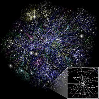
In mathematics, random graph is the general term to refer to probability distributions over graphs. Random graphs may be described simply by a probability distribution, or by a random process which generates them. The theory of random graphs lies at the intersection between graph theory and probability theory. From a mathematical perspective, random graphs are used to answer questions about the properties of typical graphs. Its practical applications are found in all areas in which complex networks need to be modeled – many random graph models are thus known, mirroring the diverse types of complex networks encountered in different areas. In a mathematical context, random graph refers almost exclusively to the Erdős–Rényi random graph model. In other contexts, any graph model may be referred to as a random graph.

<span class="mw-page-title-main">Spanning tree</span> Tree which includes all vertices of a graph

In the mathematical field of graph theory, a spanning treeT of an undirected graph G is a subgraph that is a tree which includes all of the vertices of G. In general, a graph may have several spanning trees, but a graph that is not connected will not contain a spanning tree. If all of the edges of G are also edges of a spanning tree T of G, then G is a tree and is identical to T.

In graph theory, the resistance distance between two vertices of a simple, connected graph, G, is equal to the resistance between two equivalent points on an electrical network, constructed so as to correspond to G, with each edge being replaced by a resistance of one ohm. It is a metric on graphs.

<span class="mw-page-title-main">Bethe lattice</span>

In statistical mechanics and mathematics, the Bethe lattice is an infinite connected cycle-free graph where all vertices have the same number of neighbors. The Bethe lattice was introduced into the physics literature by Hans Bethe in 1935. In such a graph, each node is connected to z neighbors; the number z is called either the coordination number or the degree, depending on the field.

<span class="mw-page-title-main">Dominating set</span> Subset of a graphs nodes such that all other nodes link to at least one

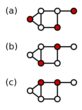
In graph theory, a dominating set for a graph G is a subset D of its vertices, such that any vertex of G is in D, or has a neighbor in D. The domination numberγ(G) is the number of vertices in a smallest dominating set for G.

In the mathematical discipline of graph theory, the expander walk sampling theorem intuitively states that sampling vertices in an expander graph by doing relatively short random walk can simulate sampling the vertices independently from a uniform distribution. The earliest version of this theorem is due to Ajtai, Komlós & Szemerédi (1987), and the more general version is typically attributed to Gillman (1998).

<span class="mw-page-title-main">Schramm–Loewner evolution</span>

In probability theory, the Schramm–Loewner evolution with parameter κ, also known as stochastic Loewner evolution (SLEκ), is a family of random planar curves that have been proven to be the scaling limit of a variety of two-dimensional lattice models in statistical mechanics. Given a parameter κ and a domain in the complex plane U, it gives a family of random curves in U, with κ controlling how much the curve turns. There are two main variants of SLE, chordal SLE which gives a family of random curves from two fixed boundary points, and radial SLE, which gives a family of random curves from a fixed boundary point to a fixed interior point. These curves are defined to satisfy conformal invariance and a domain Markov property.

<span class="mw-page-title-main">Random geometric graph</span> In graph theory, the mathematically simplest spatial network

In graph theory, a random geometric graph (RGG) is the mathematically simplest spatial network, namely an undirected graph constructed by randomly placing N nodes in some metric space and connecting two nodes by a link if and only if their distance is in a given range, e.g. smaller than a certain neighborhood radius, r.

In the mathematical subject of group theory, the Grushko theorem or the Grushko–Neumann theorem is a theorem stating that the rank of a free product of two groups is equal to the sum of the ranks of the two free factors. The theorem was first obtained in a 1940 article of Grushko and then, independently, in a 1943 article of Neumann.

<span class="mw-page-title-main">Abelian sandpile model</span> Cellular automaton

The Abelian sandpile model (ASM) is the more popular name of the original Bak–Tang–Wiesenfeld model (BTW). The BTW model was the first discovered example of a dynamical system displaying self-organized criticality. It was introduced by Per Bak, Chao Tang and Kurt Wiesenfeld in a 1987 paper.

In matroid theory, a field within mathematics, a gammoid is a certain kind of matroid, describing sets of vertices that can be reached by vertex-disjoint paths in a directed graph.

Bidimensionality theory characterizes a broad range of graph problems (bidimensional) that admit efficient approximate, fixed-parameter or kernel solutions in a broad range of graphs. These graph classes include planar graphs, map graphs, bounded-genus graphs and graphs excluding any fixed minor. In particular, bidimensionality theory builds on the graph minor theory of Robertson and Seymour by extending the mathematical results and building new algorithmic tools. The theory was introduced in the work of Demaine, Fomin, Hajiaghayi, and Thilikos, for which the authors received the Nerode Prize in 2015.

The expected linear time MST algorithm is a randomized algorithm for computing the minimum spanning forest of a weighted graph with no isolated vertices. It was developed by David Karger, Philip Klein, and Robert Tarjan. The algorithm relies on techniques from Borůvka's algorithm along with an algorithm for verifying a minimum spanning tree in linear time. It combines the design paradigms of divide and conquer algorithms, greedy algorithms, and randomized algorithms to achieve expected linear performance.

In coding theory, Zemor's algorithm, designed and developed by Gilles Zemor, is a recursive low-complexity approach to code construction. It is an improvement over the algorithm of Sipser and Spielman.

Maximal entropy random walk (MERW) is a popular type of biased random walk on a graph, in which transition probabilities are chosen accordingly to the principle of maximum entropy, which says that the probability distribution which best represents the current state of knowledge is the one with largest entropy. While standard random walk chooses for every vertex uniform probability distribution among its outgoing edges, locally maximizing entropy rate, MERW maximizes it globally by assuming uniform probability distribution among all paths in a given graph.

In graph theory a minimum spanning tree (MST) of a graph with and is a tree subgraph of that contains all of its vertices and is of minimum weight.

References