In statistics, stochastic volatility models are those in which the variance of a stochastic process is itself randomly distributed.[1] They are used in the field of mathematical finance to evaluate derivativesecurities, such as options. The name derives from the models' treatment of the underlying security's volatility as a random process, governed by state variables such as the price level of the underlying security, the tendency of volatility to revert to some long-run mean value, and the variance of the volatility process itself, among others.
Stochastic volatility models are one approach to resolve a shortcoming of the Black–Scholes model. In particular, models based on Black-Scholes assume that the underlying volatility is constant over the life of the derivative, and unaffected by the changes in the price level of the underlying security. However, these models cannot explain long-observed features of the implied volatility surface such as volatility smile and skew, which indicate that implied volatility does tend to vary with respect to strike price and expiry. By assuming that the volatility of the underlying price is a stochastic process rather than a constant, it becomes possible to model derivatives more accurately.
A middle ground between the bare Black-Scholes model and stochastic volatility models is covered by local volatility models. In these models the underlying volatility does not feature any new randomness but it isn't a constant either. In local volatility models the volatility is a non-trivial function of the underlying asset, without any extra randomness. According to this definition, models like constant elasticity of variance would be local volatility models, although they are sometimes classified as stochastic volatility models. The classification can be a little ambiguous in some cases.
The early history of stochastic volatility has multiple roots (i.e. stochastic process, option pricing and econometrics), it is reviewed in Chapter 1 of Neil Shephard (2005) "Stochastic Volatility," Oxford University Press.
Basic model
Starting from a constant volatility approach, assume that the derivative's underlying asset price follows a standard model for geometric Brownian motion:
where is the constant drift (i.e. expected return) of the security price , is the constant volatility, and is a standard Wiener process with zero mean and unit rate of variance. The explicit solution of this stochastic differential equation is
The maximum likelihood estimator to estimate the constant volatility for given stock prices at different times is
For a stochastic volatility model, replace the constant volatility with a function that models the variance of . This variance function is also modeled as Brownian motion, and the form of depends on the particular SV model under study.
where and are some functions of , and is another standard gaussian that is correlated with with constant correlation factor .
The popular Heston model is a commonly used SV model, in which the randomness of the variance process varies as the square root of variance. In this case, the differential equation for variance takes the form:
where is the mean long-term variance, is the rate at which the variance reverts toward its long-term mean, is the volatility of the variance process, and is, like , a gaussian with zero mean and variance. However, and are correlated with the constant correlation value .
In other words, the Heston SV model assumes that the variance is a random process that
exhibits a tendency to revert towards a long-term mean at a rate ,
exhibits a volatility proportional to the square root of its level
and whose source of randomness is correlated (with correlation ) with the randomness of the underlying's price processes.
Some parametrisation of the volatility surface, such as 'SVI',[2] are based on the Heston model.
The CEV model describes the relationship between volatility and price, introducing stochastic volatility:
Conceptually, in some markets volatility rises when prices rise (e.g. commodities), so . In other markets, volatility tends to rise as prices fall, modelled with .
Some argue that because the CEV model does not incorporate its own stochastic process for volatility, it is not truly a stochastic volatility model. Instead, they call it a local volatility model.
The SABR model (Stochastic Alpha, Beta, Rho), introduced by Hagan et al.[3] describes a single forward (related to any asset e.g. an index, interest rate, bond, currency or equity) under stochastic volatility :
The initial values and are the current forward price and volatility, whereas and are two correlated Wiener processes (i.e. Brownian motions) with correlation coefficient . The constant parameters are such that .
The main feature of the SABR model is to be able to reproduce the smile effect of the volatility smile.
GARCH model
The Generalized Autoregressive Conditional Heteroskedasticity (GARCH) model is another popular model for estimating stochastic volatility. It assumes that the randomness of the variance process varies with the variance, as opposed to the square root of the variance as in the Heston model. The standard GARCH(1,1) model has the following form for the continuous variance differential:[4]
The GARCH model has been extended via numerous variants, including the NGARCH, TGARCH, IGARCH, LGARCH, EGARCH, GJR-GARCH, Power GARCH, Component GARCH, etc. Strictly, however, the conditional volatilities from GARCH models are not stochastic since at time t the volatility is completely pre-determined (deterministic) given previous values.[5]
3/2 model
The 3/2 model is similar to the Heston model, but assumes that the randomness of the variance process varies with . The form of the variance differential is:
However the meaning of the parameters is different from Heston model. In this model, both mean reverting and volatility of variance parameters are stochastic quantities given by and respectively.
Rough volatility models
Using estimation of volatility from high frequency data, smoothness of the volatility process has been questioned.[6] It has been found that log-volatility behaves as a fractional Brownian motion with Hurst exponent of order , at any reasonable timescale. This led to adopting a fractional stochastic volatility (FSV) model,[7] leading to an overall Rough FSV (RFSV) where "rough" is to highlight that . The RFSV model is consistent with time series data, allowing for improved forecasts of realized volatility.[6]
Calibration and estimation
Once a particular SV model is chosen, it must be calibrated against existing market data. Calibration is the process of identifying the set of model parameters that are most likely given the observed data. One popular technique is to use maximum likelihood estimation (MLE). For instance, in the Heston model, the set of model parameters can be estimated applying an MLE algorithm such as the Powell Directed Set method to observations of historic underlying security prices.
In this case, you start with an estimate for , compute the residual errors when applying the historic price data to the resulting model, and then adjust to try to minimize these errors. Once the calibration has been performed, it is standard practice to re-calibrate the model periodically.
An alternative to calibration is statistical estimation, thereby accounting for parameter uncertainty. Many frequentist and Bayesian methods have been proposed and implemented, typically for a subset of the abovementioned models. The following list contains extension packages for the open source statistical software R that have been specifically designed for heteroskedasticity estimation. The first three cater for GARCH-type models with deterministic volatilities; the fourth deals with stochastic volatility estimation.
rugarch: ARFIMA, in-mean, external regressors and various GARCH flavors, with methods for fit, forecast, simulation, inference and plotting.[8]
fGarch: Part of the Rmetrics environment for teaching "Financial Engineering and Computational Finance".
bayesGARCH: Bayesian estimation of the GARCH(1,1) model with Student's t innovations.[9]
Many numerical methods have been developed over time and have solved pricing financial assets such as options with stochastic volatility models. A recent developed application is the local stochastic volatility model.[12] This local stochastic volatility model gives better results in pricing new financial assets such as forex options.
There are also alternate statistical estimation libraries in other languages such as Python:
PyFlux Includes Bayesian and classical inference support for GARCH and beta-t-EGARCH models.
In probability theory and statistics, a normal distribution or Gaussian distribution is a type of continuous probability distribution for a real-valued random variable. The general form of its probability density function is
The Black–Scholes or Black–Scholes–Merton model is a mathematical model for the dynamics of a financial market containing derivative investment instruments. From the parabolic partial differential equation in the model, known as the Black–Scholes equation, one can deduce the Black–Scholes formula, which gives a theoretical estimate of the price of European-style options and shows that the option has a unique price given the risk of the security and its expected return. The equation and model are named after economists Fischer Black and Myron Scholes. Robert C. Merton, who first wrote an academic paper on the subject, is sometimes also credited.
A geometric Brownian motion (GBM) (also known as exponential Brownian motion) is a continuous-time stochastic process in which the logarithm of the randomly varying quantity follows a Brownian motion (also called a Wiener process) with drift. It is an important example of stochastic processes satisfying a stochastic differential equation (SDE); in particular, it is used in mathematical finance to model stock prices in the Black–Scholes model.
In econometrics, the autoregressive conditional heteroskedasticity (ARCH) model is a statistical model for time series data that describes the variance of the current error term or innovation as a function of the actual sizes of the previous time periods' error terms; often the variance is related to the squares of the previous innovations. The ARCH model is appropriate when the error variance in a time series follows an autoregressive (AR) model; if an autoregressive moving average (ARMA) model is assumed for the error variance, the model is a generalized autoregressive conditional heteroskedasticity (GARCH) model.
A variance swap is an over-the-counter financial derivative that allows one to speculate on or hedge risks associated with the magnitude of movement, i.e. volatility, of some underlying product, like an exchange rate, interest rate, or stock index.
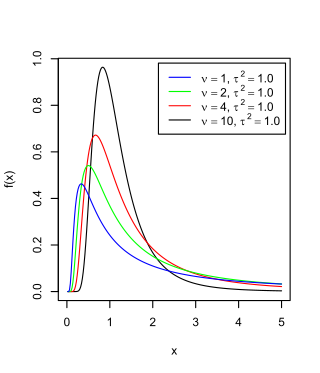
The scaled inverse chi-squared distribution is the distribution for x = 1/s2, where s2 is a sample mean of the squares of ν independent normal random variables that have mean 0 and inverse variance 1/σ2 = τ2. The distribution is therefore parametrised by the two quantities ν and τ2, referred to as the number of chi-squared degrees of freedom and the scaling parameter, respectively.
In mathematics, the Ornstein–Uhlenbeck process is a stochastic process with applications in financial mathematics and the physical sciences. Its original application in physics was as a model for the velocity of a massive Brownian particle under the influence of friction. It is named after Leonard Ornstein and George Eugene Uhlenbeck.
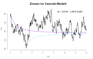
In finance, the Vasicek model is a mathematical model describing the evolution of interest rates. It is a type of one-factor short-rate model as it describes interest rate movements as driven by only one source of market risk. The model can be used in the valuation of interest rate derivatives, and has also been adapted for credit markets. It was introduced in 1977 by Oldřich Vašíček, and can be also seen as a stochastic investment model.
In finance, a volatility swap is a forward contract on the future realised volatility of a given underlying asset. Volatility swaps allow investors to trade the volatility of an asset directly, much as they would trade a price index. Its payoff at expiration is equal to
In finance, the Heston model, named after Steven L. Heston, is a mathematical model that describes the evolution of the volatility of an underlying asset. It is a stochastic volatility model: such a model assumes that the volatility of the asset is not constant, nor even deterministic, but follows a random process.
A local volatility model, in mathematical finance and financial engineering, is an option pricing model that treats volatility as a function of both the current asset level and of time . As such, it is a generalisation of the Black–Scholes model, where the volatility is a constant. Local volatility models are often compared with stochastic volatility models, where the instantaneous volatility is not just a function of the asset level but depends also on a new "global" randomness coming from an additional random component.
Financial models with long-tailed distributions and volatility clustering have been introduced to overcome problems with the realism of classical financial models. These classical models of financial time series typically assume homoskedasticity and normality cannot explain stylized phenomena such as skewness, heavy tails, and volatility clustering of the empirical asset returns in finance. In 1963, Benoit Mandelbrot first used the stable distribution to model the empirical distributions which have the skewness and heavy-tail property. Since -stable distributions have infinite -th moments for all , the tempered stable processes have been proposed for overcoming this limitation of the stable distribution.
In the theory of stochastic processes, a part of the mathematical theory of probability, the variance gamma (VG) process, also known as Laplace motion, is a Lévy process determined by a random time change. The process has finite moments, distinguishing it from many Lévy processes. There is no diffusion component in the VG process and it is thus a pure jump process. The increments are independent and follow a variance-gamma distribution, which is a generalization of the Laplace distribution.
In financial econometrics, the Markov-switching multifractal (MSM) is a model of asset returns developed by Laurent E. Calvet and Adlai J. Fisher that incorporates stochastic volatility components of heterogeneous durations. MSM captures the outliers, log-memory-like volatility persistence and power variation of financial returns. In currency and equity series, MSM compares favorably with standard volatility models such as GARCH(1,1) and FIGARCH both in- and out-of-sample. MSM is used by practitioners in the financial industry to forecast volatility, compute value-at-risk, and price derivatives.
Realized variance or realised variance is the sum of squared returns. For instance the RV can be the sum of squared daily returns for a particular month, which would yield a measure of price variation over this month. More commonly, the realized variance is computed as the sum of squared intraday returns for a particular day.
In mathematical finance, the CEV or constant elasticity of variance model is a stochastic volatility model that attempts to capture stochastic volatility and the leverage effect. The model is widely used by practitioners in the financial industry, especially for modelling equities and commodities. It was developed by John Cox in 1975.
In statistics, the variance function is a smooth function that depicts the variance of a random quantity as a function of its mean. The variance function is a measure of heteroscedasticity and plays a large role in many settings of statistical modelling. It is a main ingredient in the generalized linear model framework and a tool used in non-parametric regression, semiparametric regression and functional data analysis. In parametric modeling, variance functions take on a parametric form and explicitly describe the relationship between the variance and the mean of a random quantity. In a non-parametric setting, the variance function is assumed to be a smooth function.
An additive process, in probability theory, is a cadlag, continuous in probability stochastic process with independent increments. An additive process is the generalization of a Lévy process. An example of an additive process that is not a Lévy process is a Brownian motion with a time-dependent drift. The additive process was introduced by Paul Lévy in 1937.
In finance, an option on realized variance is a type of variance derivatives which is the derivative securities on which the payoff depends on the annualized realized variance of the return of a specified underlying asset, such as stock index, bond, exchange rate, etc. Another liquidated security of the same type is variance swap, which is, in other words, the futures contract on realized variance.
In statistics, the Innovation Method provides an estimator for the parameters of stochastic differential equations given a time series of observations of the state variables. In the framework of continuous-discrete state space models, the innovation estimator is obtained by maximizing the log-likelihood of the corresponding discrete-time innovation process with respect to the parameters. The innovation estimator can be classified as a M-estimator, a quasi-maximum likelihood estimator or a prediction error estimator depending on the inferential considerations that want to be emphasized. The innovation method is a system identification technique for developing mathematical models of dynamical systems from measured data and for the optimal design of experiments.
This page is based on this Wikipedia article Text is available under the CC BY-SA 4.0 license; additional terms may apply. Images, videos and audio are available under their respective licenses.