In particle physics, the Dirac equation is a relativistic wave equation derived by British physicist Paul Dirac in 1928. In its free form, or including electromagnetic interactions, it describes all spin-1⁄2 massive particles, called "Dirac particles", such as electrons and quarks for which parity is a symmetry. It is consistent with both the principles of quantum mechanics and the theory of special relativity, and was the first theory to account fully for special relativity in the context of quantum mechanics. It was validated by accounting for the fine structure of the hydrogen spectrum in a completely rigorous way.

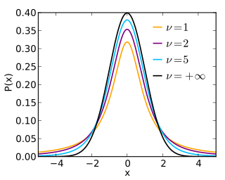
In probability and statistics, Student's t-distribution is any member of a family of continuous probability distributions that arise when estimating the mean of a normally distributed population in situations where the sample size is small and the population's standard deviation is unknown. It was developed by English statistician William Sealy Gosset under the pseudonym "Student".

In probability theory and statistics, the Weibull distribution is a continuous probability distribution. It is named after Swedish mathematician Waloddi Weibull, who described it in detail in 1951, although it was first identified by Maurice René Fréchet and first applied by Rosin & Rammler (1933) to describe a particle size distribution.
In statistics, econometrics and signal processing, an autoregressive (AR) model is a representation of a type of random process; as such, it is used to describe certain time-varying processes in nature, economics, etc. The autoregressive model specifies that the output variable depends linearly on its own previous values and on a stochastic term ; thus the model is in the form of a stochastic difference equation. Together with the moving-average (MA) model, it is a special case and key component of the more general autoregressive–moving-average (ARMA) and autoregressive integrated moving average (ARIMA) models of time series, which have a more complicated stochastic structure; it is also a special case of the vector autoregressive model (VAR), which consists of a system of more than one interlocking stochastic difference equation in more than one evolving random variable.
An activity coefficient is a factor used in thermodynamics to account for deviations from ideal behaviour in a mixture of chemical substances. In an ideal mixture, the microscopic interactions between each pair of chemical species are the same and, as a result, properties of the mixtures can be expressed directly in terms of simple concentrations or partial pressures of the substances present e.g. Raoult's law. Deviations from ideality are accommodated by modifying the concentration by an activity coefficient. Analogously, expressions involving gases can be adjusted for non-ideality by scaling partial pressures by a fugacity coefficient.
In probability theory and statistics, the generalized extreme value (GEV) distribution is a family of continuous probability distributions developed within extreme value theory to combine the Gumbel, Fréchet and Weibull families also known as type I, II and III extreme value distributions. By the extreme value theorem the GEV distribution is the only possible limit distribution of properly normalized maxima of a sequence of independent and identically distributed random variables. Note that a limit distribution needs to exist, which requires regularity conditions on the tail of the distribution. Despite this, the GEV distribution is often used as an approximation to model the maxima of long (finite) sequences of random variables.

The scaled inverse chi-squared distribution is the distribution for x = 1/s2, where s2 is a sample mean of the squares of ν independent normal random variables that have mean 0 and inverse variance 1/σ2 = τ2. The distribution is therefore parametrised by the two quantities ν and τ2, referred to as the number of chi-squared degrees of freedom and the scaling parameter, respectively.

In probability theory and statistics, the chi distribution is a continuous probability distribution. It is the distribution of the positive square root of the sum of squares of a set of independent random variables each following a standard normal distribution, or equivalently, the distribution of the Euclidean distance of the random variables from the origin. It is thus related to the chi-squared distribution by describing the distribution of the positive square roots of a variable obeying a chi-squared distribution.

In mathematics, the Ornstein–Uhlenbeck process is a stochastic process with applications in financial mathematics and the physical sciences. Its original application in physics was as a model for the velocity of a massive Brownian particle under the influence of friction. It is named after Leonard Ornstein and George Eugene Uhlenbeck.
In statistics, stochastic volatility models are those in which the variance of a stochastic process is itself randomly distributed. They are used in the field of mathematical finance to evaluate derivative securities, such as options. The name derives from the models' treatment of the underlying security's volatility as a random process, governed by state variables such as the price level of the underlying security, the tendency of volatility to revert to some long-run mean value, and the variance of the volatility process itself, among others.
Expected shortfall (ES) is a risk measure—a concept used in the field of financial risk measurement to evaluate the market risk or credit risk of a portfolio. The "expected shortfall at q% level" is the expected return on the portfolio in the worst of cases. ES is an alternative to value at risk that is more sensitive to the shape of the tail of the loss distribution.
A ratio distribution is a probability distribution constructed as the distribution of the ratio of random variables having two other known distributions. Given two random variables X and Y, the distribution of the random variable Z that is formed as the ratio Z = X/Y is a ratio distribution.
In finance, a volatility swap is a forward contract on the future realised volatility of a given underlying asset. Volatility swaps allow investors to trade the volatility of an asset directly, much as they would trade a price index. Its payoff at expiration is equal to
Tail value at risk (TVaR), also known as tail conditional expectation (TCE) or conditional tail expectation (CTE), is a risk measure associated with the more general value at risk. It quantifies the expected value of the loss given that an event outside a given probability level has occurred.
In probability and statistics, the Tweedie distributions are a family of probability distributions which include the purely continuous normal, gamma and inverse Gaussian distributions, the purely discrete scaled Poisson distribution, and the class of compound Poisson–gamma distributions which have positive mass at zero, but are otherwise continuous. Tweedie distributions are a special case of exponential dispersion models and are often used as distributions for generalized linear models.
Financial models with long-tailed distributions and volatility clustering have been introduced to overcome problems with the realism of classical financial models. These classical models of financial time series typically assume homoskedasticity and normality cannot explain stylized phenomena such as skewness, heavy tails, and volatility clustering of the empirical asset returns in finance. In 1963, Benoit Mandelbrot first used the stable distribution to model the empirical distributions which have the skewness and heavy-tail property. Since -stable distributions have infinite -th moments for all , the tempered stable processes have been proposed for overcoming this limitation of the stable distribution.

In probability theory and directional statistics, a wrapped normal distribution is a wrapped probability distribution that results from the "wrapping" of the normal distribution around the unit circle. It finds application in the theory of Brownian motion and is a solution to the heat equation for periodic boundary conditions. It is closely approximated by the von Mises distribution, which, due to its mathematical simplicity and tractability, is the most commonly used distribution in directional statistics.
The Gent hyperelastic material model is a phenomenological model of rubber elasticity that is based on the concept of limiting chain extensibility. In this model, the strain energy density function is designed such that it has a singularity when the first invariant of the left Cauchy-Green deformation tensor reaches a limiting value .
In mathematical finance, the CEV or constant elasticity of variance model is a stochastic volatility model that attempts to capture stochastic volatility and the leverage effect. The model is widely used by practitioners in the financial industry, especially for modelling equities and commodities. It was developed by John Cox in 1975.
In mathematical physics, the Gordon decomposition of the Dirac current is a splitting of the charge or particle-number current into a part that arises from the motion of the center of mass of the particles and a part that arises from gradients of the spin density. It makes explicit use of the Dirac equation and so it applies only to "on-shell" solutions of the Dirac equation.


