Gaussian filter

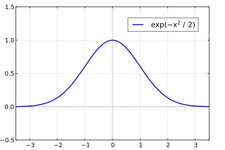
Shape of the impulse response of a typical Gaussian filter

In electronics and signal processing, mainly in digital signal processing, a Gaussian filter is a filter whose impulse response is a Gaussian function (or an approximation to it, since a true Gaussian response would have infinite impulse response). Gaussian filters have the properties of having no overshoot to a step function input while minimizing the rise and fall time. This behavior is closely connected to the fact that the Gaussian filter has the minimum possible group delay. A Gaussian filter will have the best combination of suppression of high frequencies while also minimizing spatial spread, being the critical point of the uncertainty principle. These properties are important in areas such as oscilloscopes ^[1] and digital telecommunication systems. ^[2]

Mathematically, a Gaussian filter modifies the input signal by convolution with a Gaussian function; this transformation is also known as the Weierstrass transform.

Definition

The one-dimensional Gaussian filter has an impulse response given by

${\displaystyle g(x)={\sqrt {\frac {a}{\pi }}}e^{-ax^{2}}}$

and the frequency response is given by the Fourier transform

${\displaystyle {\hat {g}}(f)=e^{-\pi ^{2}f^{2}/a}}$

with ${\displaystyle f}$ the ordinary frequency. These equations can also be expressed with the standard deviation as parameter

${\displaystyle g(x)={\frac {1}{{\sqrt {2\pi }}\sigma }}e^{-x^{2}/(2\sigma ^{2})}}$

and the frequency response is given by

${\displaystyle {\hat {g}}(f)=e^{-f^{2}/(2\sigma _{f}^{2})}}$

By writing ${\displaystyle a}$ as a function of ${\displaystyle \sigma }$ with the two equations for ${\displaystyle g(x)}$ and as a function of ${\displaystyle \sigma _{f}}$ with the two equations for ${\displaystyle {\hat {g}}(f)}$ it can be shown that the product of the standard deviation and the standard deviation in the frequency domain is given by

${\displaystyle \sigma \sigma _{f}={\frac {1}{2\pi }}}$,

where the standard deviations are expressed in their physical units, e.g. in the case of time and frequency in seconds and hertz, respectively.

In two dimensions, it is the product of two such Gaussians, one per direction:

${\displaystyle g(x,y)={\frac {1}{2\pi \sigma ^{2}}}e^{-(x^{2}+y^{2})/(2\sigma ^{2})}}$ ^{[3] [4] [5]}

where x is the distance from the origin in the horizontal axis, y is the distance from the origin in the vertical axis, and σ is the standard deviation of the Gaussian distribution.

Synthesizing Gaussian filter polynomials

The Gaussian transfer function polynomials may be synthesized using a Taylor series expansion of the square of Gaussian function of the form ${\displaystyle \epsilon ^{-a\omega ^{2}}}$ where ${\displaystyle a}$ is set such that ${\displaystyle \epsilon ^{-a\omega ^{2}}={\sqrt {1/2}}}$ (equivalent of -3.01dB) at ${\displaystyle \omega =1}$. ^[6] The value of ${\displaystyle a}$ may be calculated with this constraint to be ${\displaystyle a=-log{\bigg (}{\sqrt {1/2}}{\bigg )}}$, or 0.34657359 for an approximate -3.010 dB cutoff attenuation. If an attenuation of other than -3.010 dB is desired,${\displaystyle a}$ may be recalculated using a different attenuation, ${\displaystyle a=log(10^{(|dB|/20)})}$.

To meet all above criteria, ${\displaystyle F(\omega )}$ must be of the form obtained below, with no stop band zeros,

${\displaystyle F(\omega )=\epsilon ^{-a\omega ^{2}}{\sqrt {(\epsilon ^{-a\omega ^{2}})^{2}}}={\sqrt {\frac {1}{\epsilon ^{2a\omega ^{2}}}}}}$

To complete the transfer function, ${\displaystyle \epsilon ^{2a\omega ^{2}}}$may be approximated with a Taylor Series expansion about 0. The full Taylor series for ${\displaystyle \epsilon ^{2a\omega ^{2}}}$ is shown below. ^[6]

${\displaystyle \epsilon ^{2a\omega ^{2}}=\sum _{k=0}^{\infty }{\frac {(2a)^{k}\omega ^{2k}}{k!}}}$

The ability of the filter to simulate a true Gaussian function depends on how many terms are taken from the series. The number of terms taken beyond 0 establishes the order N of the filter.

${\displaystyle F_{N}(\omega )={\sqrt {\frac {1}{\sum _{k=0}^{\mathbb {N} }{\frac {(2a)^{k}\omega ^{2k}}{k!}}}}}}$

For the frequency axis, ${\displaystyle \omega }$ is replace with ${\displaystyle j\omega }$.

${\displaystyle F_{N}(j\omega )={\sqrt {\frac {1}{\sum _{k=0}^{\mathbb {N} }{\frac {(2a)^{k}(j\omega )^{2k}}{k!}}}}}{\bigg |}_{\text{left half plane}}}$

Since only half the poles are located in the left half plane, selecting only those poles to build the transfer function also serves to square root the equation, as is seen above.

Simple 3rd order example

A 3rd order Gaussian filter with a -3.010 dB cutoff attenuation at ${\displaystyle \omega }$ = 1 requires the use of terms k=0 to k=3 in the Taylor series to produce the squared Gaussian function.

${\displaystyle F_{3}((j\omega )^{2})={\frac {1}{1.33333a^{3}(j\omega )^{6}+2a^{2}(j\omega ^{4})+2a(j\omega )^{2}+1}}={\frac {1}{-1.33333a^{3}\omega ^{6}+2a^{2}\omega ^{4}-2a\omega ^{2}+1}}}$

Absorbing ${\displaystyle a}$ into the coefficients, factoring using a root finding algorithm, and building the polynomials using only the left half plane poles yields the transfer function for a third order Gaussian filter with the required -3.010 dB cutoff attenuation ^{[7] [8]} ..

${\displaystyle F_{3}(j\omega )={\frac {1}{0.2355931(j\omega )^{3}+1.0078328(j\omega )^{2}+1.6458471(j\omega )+1}}}$

A quick sanity check of evaluating ${\displaystyle |F_{3}(j)|}$ yields a magnitude of -2.986 dB, which represents an error of only ~0.8% from the desired -3.010 dB. This error will decrease as the number of orders increases. In addition, the error at higher frequencies will be more pronounced for all Gaussian filters, bug will also decrease as the order of the filter increases. ^[6]

Gaussian Transitional Filters

Although Gaussian filters exhibit desirable group delay, as described in the opening description, the steepness of the cutoff attenuation may be less than desired. ^[9] To work around this, tables have been developed and published that preserve the desirable Gaussian group delay response ant the lower and mid frequencies, and then switch to a higher steepness Chebyshev attenuation at the higher frequencies. ^[9]

Digital implementation

The Gaussian function is for ${\displaystyle x\in (-\infty ,\infty )}$ and would theoretically require an infinite window length. However, since it decays rapidly, it is often reasonable to truncate the filter window and implement the filter directly for narrow windows, in effect by using a simple rectangular window function. In other cases, the truncation may introduce significant errors. Better results can be achieved by instead using a different window function; see scale space implementation for details.

Filtering involves convolution. The filter function is said to be the kernel of an integral transform. The Gaussian kernel is continuous. Most commonly, the discrete equivalent is the sampled Gaussian kernel that is produced by sampling points from the continuous Gaussian. An alternate method is to use the discrete Gaussian kernel ^[10] which has superior characteristics for some purposes. Unlike the sampled Gaussian kernel, the discrete Gaussian kernel is the solution to the discrete diffusion equation.

Since the Fourier transform of the Gaussian function yields a Gaussian function, the signal (preferably after being divided into overlapping windowed blocks) can be transformed with a fast Fourier transform, multiplied with a Gaussian function and transformed back. This is the standard procedure of applying an arbitrary finite impulse response filter, with the only difference being that the Fourier transform of the filter window is explicitly known.

Due to the central limit theorem (from statistics), the Gaussian can be approximated by several runs of a very simple filter such as the moving average. The simple moving average corresponds to convolution with the constant B-spline (a rectangular pulse). For example, four iterations of a moving average yield a cubic B-spline as a filter window, which approximates the Gaussian quite well. A moving average is quite cheap to compute, so levels can be cascaded quite easily.

In the discrete case, the filter's standard deviations (in the time and frequency domains) are related by

${\displaystyle \sigma _{t}\cdot \sigma _{f}={\frac {N}{2\pi }}}$

where the standard deviations are expressed in a number of samples and N is the total number of samples. The standard deviation of a filter can be interpreted as a measure of its size. The cut-off frequency of a Gaussian filter might be defined by the standard deviation in the frequency domain:

${\displaystyle f_{c}=\sigma _{f}={\frac {1}{2\pi \sigma _{t}}}}$

where all quantities are expressed in their physical units. If ${\displaystyle \sigma _{t}}$ is measured in samples, the cut-off frequency (in physical units) can be calculated with

${\displaystyle f_{c}={\frac {F_{s}}{2\pi \sigma _{t}}}}$

where ${\displaystyle F_{s}}$ is the sample rate. The response value of the Gaussian filter at this cut-off frequency equals exp(−0.5) ≈ 0.607.

However, it is more common to define the cut-off frequency as the half power point: where the filter response is reduced to 0.5 (−3 dB) in the power spectrum, or 1/√2 ≈ 0.707 in the amplitude spectrum (see e.g. Butterworth filter). For an arbitrary cut-off value 1/c for the response of the filter, the cut-off frequency is given by

${\displaystyle f_{c}={\sqrt {2\ln(c)}}\cdot \sigma _{f}}$ ^[11]

For c = 2 the constant before the standard deviation in the frequency domain in the last equation equals approximately 1.1774, which is half the Full Width at Half Maximum (FWHM) (see Gaussian function). For c = √2 this constant equals approximately 0.8326. These values are quite close to 1.

A simple moving average corresponds to a uniform probability distribution and thus its filter width of size ${\displaystyle n}$ has standard deviation ${\displaystyle {\sqrt {(n^{2}-1)/12}}}$. Thus the application of successive ${\displaystyle m}$ moving averages with sizes ${\displaystyle {n}_{1},\dots ,{n}_{m}}$ yield a standard deviation of

${\displaystyle \sigma ={\sqrt {\frac {n_{1}^{2}+\cdots +n_{m}^{2}-m}{12}}}}$

(Note that standard deviations do not sum up, but variances do.)

A gaussian kernel requires ${\displaystyle 6\sigma _{t}-1}$ values, e.g. for a ${\displaystyle {\sigma _{t}}}$ of 3, it needs a kernel of length 17. A running mean filter of 5 points will have a sigma of ${\displaystyle {\sqrt {2}}}$. Running it three times will give a ${\displaystyle {\sigma _{t}}}$ of 2.42. It remains to be seen where the advantage is over using a gaussian rather than a poor approximation.

When applied in two dimensions, this formula produces a Gaussian surface that has a maximum at the origin, whose contours are concentric circles with the origin as center. A two-dimensional convolution matrix is precomputed from the formula and convolved with two-dimensional data. Each element in the resultant matrix new value is set to a weighted average of that element's neighborhood. The focal element receives the heaviest weight (having the highest Gaussian value), and neighboring elements receive smaller weights as their distance to the focal element increases. In Image processing, each element in the matrix represents a pixel attribute such as brightness or color intensity, and the overall effect is called Gaussian blur.

The Gaussian filter is non-causal, which means the filter window is symmetric about the origin in the time domain. This makes the Gaussian filter physically unrealizable. This is usually of no consequence for applications where the filter bandwidth is much larger than the signal. In real-time systems, a delay is incurred because incoming samples need to fill the filter window before the filter can be applied to the signal. While no amount of delay can make a theoretical Gaussian filter causal (because the Gaussian function is non-zero everywhere), the Gaussian function converges to zero so rapidly that a causal approximation can achieve any required tolerance with a modest delay, even to the accuracy of floating point representation.

Applications

• GSM since it applies GMSK modulation
• the Gaussian filter is also used in GFSK.
• Canny Edge Detector used in image processing.

See also

• Butterworth filter
• Comb filter
• Chebyshev filter
• Discrete Gaussian kernel
• Elliptic filter
• Gaussian blur
• Gaussian pyramid
• Scale space
• Scale space implementation

References

1. Orwiler, Bob (1969). Oscilloscope Vertical Amplifiers (PDF) (1 ed.). Beaverton, Oregon: Tektronix Circuit Concepts. Archived (PDF) from the original on 14 October 2011. Retrieved 17 November 2022.
2. Andrews, James R (1999). "Low-Pass Risetime Filters for Time Domain Applications" (PDF). kh6htv.com. Picosecond Pulse Labs. Archived (PDF) from the original on 21 July 2016. Retrieved 17 November 2022.
3. R.A. Haddad and A.N. Akansu, "A Class of Fast Gaussian Binomial Filters for Speech and Image Processing," IEEE Transactions on Acoustics, Speech, and Signal Processing, vol. 39, pp 723–727, March 1991.
4. Shapiro, L. G. & Stockman, G. C: "Computer Vision", page 137, 150. Prentence Hall, 2001
5. Mark S. Nixon and Alberto S. Aguado. Feature Extraction and Image Processing. Academic Press, 2008, p. 88.
6. Zverev, Anatol I. (1967). Handbook of Filter Synthesis. New York, Chichester, Brisbane, Toronto, Singapore: John Wiley & Sons, Inc. pp. 70, 71. ISBN   0 471 98680 1.
7. Dr. Byron Bennett's filter design lecture notes, 1985, Montana State University, EE Department, Bozeman, Montana, US
8. Sedra, Adel S.; Brackett, Peter O. (1978). Filter Theory and Design: Active and Passive. Beaverton, Oegon, US: Matrix Publishers, Inc. pp. 45–73. ISBN   978-0916460143.
9. Williams, Arthur Bernard; Taylor, Fred J. (1995). Electronic Filter Design Handbook (3rd ed.). US: McGraw-Hill, Inc. pp. 2.56, 2.65, 11.62. ISBN   0-07-070441-4.
10. Lindeberg, T., "Scale-space for discrete signals," PAMI(12), No. 3, March 1990, pp. 234–254.
11. Stefano Bottacchi, Noise and Signal Interference in Optical Fiber Transmission Systems, p. 242, John Wiley & Sons, 2008 ISBN   047051681X