Chebyshev filters are analog or digital filters that have a steeper roll-off than Butterworth filters, and have either passbandripple (type I) or stopband ripple (type II). Chebyshev filters have the property that they minimize the error between the idealized and the actual filter characteristic over the operating frequency range of the filter,[1][2] but they achieve this with ripples in the passband. This type of filter is named after Pafnuty Chebyshev because its mathematical characteristics are derived from Chebyshev polynomials. Type I Chebyshev filters are usually referred to as "Chebyshev filters", while type II filters are usually called "inverse Chebyshev filters".[3] Because of the passband ripple inherent in Chebyshev filters, filters with a smoother response in the passband but a more irregular response in the stopband are preferred for certain applications.[4]
The frequency response of a fourth-order type I Chebyshev low-pass filter with
Type I Chebyshev filters are the most common types of Chebyshev filters. The gain (or amplitude) response, , as a function of angular frequency of the th-order low-pass filter is equal to the absolute value of the transfer function evaluated at :
The passband exhibits equiripple behavior, with the ripple determined by the ripple factor . In the passband, the Chebyshev polynomial alternates between -1 and 1 so the filter gain alternate between maxima at and minima at .
The ripple factor ε is thus related to the passband ripple δ in decibels by:
At the cutoff frequency the gain again has the value but continues to drop into the stopband as the frequency increases. This behavior is shown in the diagram on the right. The common practice of defining the cutoff frequency at −3dB is usually not applied to Chebyshev filters; instead the cutoff is taken as the point at which the gain falls to the value of the ripple for the final time.
The 3dB frequency is related to by:
The order of a Chebyshev filter is equal to the number of reactive components (for example, inductors) needed to realize the filter using analog electronics.
An even steeper roll-off can be obtained if ripple is allowed in the stopband, by allowing zeros on the -axis in the complex plane. While this produces near-infinite suppression at and near these zeros (limited by the quality factor of the components, parasitics, and related factors), overall suppression in the stopband is reduced. The result is called an elliptic filter, also known as a Cauer filter.
Poles and zeroes
Log of the absolute value of the gain of an 8th-order Chebyshev type I filter in complex frequency space (s=σ+jω) with ε=0.1 and . The white spots are poles and are arranged on an ellipse with a semi-axis of 0.3836... in σ and 1.071... in ω. The transfer function poles are those poles in the left half plane. Black corresponds to a gain of 0.05 or less, white corresponds to a gain of 20 or more.
For simplicity, it is assumed that the cutoff frequency is equal to unity. The poles of the gain function of the Chebyshev filter are the zeroes of the denominator of the gain function. Using the complex frequency , these occur when:
Defining and using the trigonometric definition of the Chebyshev polynomials yields:
Solving for
where the multiple values of the arc cosine function are made explicit using the integer index . The poles of the Chebyshev gain function are then:
Using the properties of the trigonometric and hyperbolic functions, this may be written in explicitly complex form:
where and
This may be viewed as an equation parametric in and it demonstrates that the poles lie on an ellipse in -space centered at with a real semi-axis of length and an imaginary semi-axis of length of
The transfer function
The above expression yields the poles of the gain . For each complex pole, there is another which is the complex conjugate, and for each conjugate pair there are two more that are the negatives of the pair. The transfer function must be stable, so that its poles are those of the gain that have negative real parts and therefore lie in the left half plane of complex frequency space. The transfer function is then given by
where are only those poles of the gain with a negative sign in front of the real term, obtained from the above equation.
The group delay
Gain and group delay of a 5th-order type I Chebyshev filter with ε = 0.5.
The group delay is defined as the derivative of the phase with respect to angular frequency:
The gain and the group delay for a 5th-order type I Chebyshev filter with ε=0.5 are plotted in the graph on the left. It's stop band has no ripples. But the ripples of group delay in its passband indicate that different frequency components have different delay, which along with the ripples of gain in its passband results in distortion of the waveform's shape.
Even order modifications
Even order Chebyshev filters implemented with passive elements, typically inductors, capacitors, and transmission lines, with terminations of equal value on each side cannot be implemented with the traditional Chebyshev transfer function without the use of coupled coils, which may not be desirable or feasible. This is due to the physical inability to accommodate the even order Chebyshev reflection zeros that result in a scattering matrix S12 values that exceed the S12 value at . If it is not feasible to design the filter with one of the terminations increased or decreased to accommodate the pass band S12, then the Chebyshev transfer function must be modified so as to move the lowest even order reflection zero to while maintaining the equi-ripple response of the pass band.[5]
The needed modification involves mapping each pole of the Chebyshev transfer function in a manner that maps the lowest frequency reflection zero to zero and the remaining poles as needed to maintain the equi-ripple pass band. The lowest frequency reflection zero may be found from the Chebyshev Nodes, . The complete Chebyshev pole mapping function is shown below.[5]
Where:
n is the order of the filter (must be even)
P is a traditional Chebyshev transfer function pole
P' is the mapped pole for the modified even order transfer function.
"Left Half Plane" indicates to use the square root containing a negative real value.
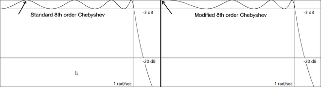
When complete, a replacement equi-ripple transfer function is created with reflection zero scattering matrix values for S12 of one and S11 of zero when implemented with equally terminated passive networks. The illustration below shows an 8th order Chebyshev filter modified to support even order equally terminated passive networks by relocating the lowest frequency reflection zero from a finite frequency to 0 while maintaining an equi-ripple pass band frequency response.
Even order modified Chebyshev illustration
The LC element value formulas in the Cauer topology are not applicable to the even order modified Chebyshev transfer function, and cannot be used. It is therefore necessary to calculate the LC values from traditional continued fractions of the impedance function, which may be derived from the reflection coefficient, which in turn may be derived from the transfer function.
Minimum order
To design a Chebyshev filter using the minimum required number of elements, the minimum order of the Chebyshev filter may be calculated as follows.[6] The equations account for standard low pass Chebyshev filters, only. Even order modifications and finite stop band transmission zeros will introduce error that the equations do not account for.
where:
and are the pass band ripple frequency and maximum ripple attenuation in dB
and are the stop band frequency and attenuation at that frequency in dB
is the minimum number of poles, the order of the filter.
ceil[] is a round up to next integer function.
Setting the cutoff attenuation
Pass band cutoff attenuation for Chebyshev filters is usually the same as the pass band ripple attenuation, set by the computation above. However, many applications such as diplexers and triplexers,[5] require a cutoff attenuation of -3.0103 dB in order to obtain the needed reflections. Other specialized applications may require other specific values for cutoff attenuation for various reasons. It is therefore useful to have a means available of setting the Chebyshev pass band cutoff attenuation independently of the pass band ripple attenuation, such as -1 dB, -10 dB, etc. The cutoff attenuation may be set by frequency scaling the poles of the transfer function.
The scaling factor may be determined by direct algebraic manipulation of the defining Chebyshev filter function, , including and . The general definition of the Chebyshev function, is required, which may be derived from the Chebyshev Polynomials equations, and the inverse Chebyshev function, . To keep the numbers real for values of , complex hyperbolic identities may be used to rewrite the equations as, and .
Using simple algebra on the above equations and references, the expression to scale each Chebyshev poles is:
Where:
is the relocated pole positioned to set the desired cutoff attenuation.
is a ripple cutoff pole that lies on the oval.
is the passband attenuation ripple in dB (.05 dB, 1 dB, etc.)).
is the desired passband attenuation at the cutoff frequency in dB (1 dB, 3 dB, 10 dB, etc.)
is the number of poles (the order of the filter).
A quick sanity check on the above equation using passband ripple attenuation for the passband cutoff attenuation reveals that the pole adjustment will be 1.0 for this case, which is what is expected.
Even order modified cutoff attenuation adjustment
For Chebyshev filters being designed with modified for even order pass band ripple for passive equally terminated filters, the attenuation frequency computation needs to include the even order adjustment by performing the even order adjustment operation on the computed attenuation frequency. This makes the even order adjustment arithmetic slightly simpler, since frequency can be treated as a real variable, in this case .
Where:
is the relocated pole positioned to set the desired cutoff attenuation.
is a ripple cutoff pole that has been modified for even order pass bands.
is the passband attenuation ripple in dB (.05 dB, 1 dB, etc.)).
is the desired passband attenuation at the cutoff frequency in dB (1 dB, 3 dB, 10 dB, etc.)
Chebyshev filters may be designed with arbitrarily placed finite transmission zeros in the stop band while retaining an equi-ripple pass band. Stop band zeros along the axis are generally used to eliminate unwanted frequencies. Stop band zeros along the real axis or quadruplet stop band zeros in the complex plane may be used to modify the group delay to a more desirable shape. The transmission zeros design utilizes characteristic polynomials, K(S), to place the transmission and reflection zeros, which in turn are used to create the transfer function, ,[7]
The calculation of K(S) relies upon the following observed equality.[7]
for all , imaginary conjugate pairs, quadruplet conjugate pairs, or real opposing signed pairs.
Given the magnitude is always one in the pass bane () the rational and irrational terms must vary between 0 and 1. Therefore, if only the rational term is used to create the characteristic function, an equi-ripple response is expected in the pass band, and characteristic poles (transmission zeros) are expected at all .
The design process for K(S) using the above expression is below.
Use the positive solution for real and imaginary pairs. Use the positive real and conjugate imaginary solution for quadruplet complex pairs.
should be normalized such that , if needed.
The, "rational terms only" indicates to keep the rational part of the product, and to discard the irrational part. The rational term may be obtained by manually performing the polynomial arithmetic, or with the short cut below which is a solution derived from polynomial arithmetic and uses binomial coefficients. The algorithm is extremely efficient if the Binomial coefficients are implemented from a look-up table of pre-calculated values.
When all M values are set to one, then will be the standard Chebyshev equation, which is expected since the all transmission zeros are it . It is also important to remember that even order finite transmission zero Chebyshev filters have the same limitation as the all-pole case in that they cannot be constructed using equally terminated passive networks. The same even order modification may be made to the even order characteristic polynomials, , to make equally terminated passive network implementations possible. However, the even order modification will also move the finite transmission zeros slightly. This movement may be significantly mitigated by propositioning the transmission zeros with the inverse of the even order modification using the lowest Chebyshev node, .
Simple example
Design a 3 pole Chebyshev filter with a 1 dB pass band, a transmission zero at 2 rad/sec, and a transmission zero at :
To find the transfer function, do the following.[7][8]
To obtain from the left half plane, factor the numerator and denominator to obtain the roots. Discard all roots from the right half plane of the denominator, half the repeated roots in the numerator, and rebuild with the remaining roots. Generally, normalize to 1 at .
To confirm that the example is correct, the plot of along is shown below with a pass band ripple of 1 dB, a cut off frequency of 1 rad/sec, and a stop band zero at 2 rad/sec.
Chebyshev transmission zero at 2 rad/sec
Asymmetric band pass filter
Chebyshev band pass filters may be designed with a geometrically asymmetric frequency response by placing the desired number of transmission zeros at zero and infinity with the use of the more generalized form of the Chebyshev transmission zeros equation above,[7] and shown below. The equations below consider a frequency normalized pass band from 1 to . If the number of transmission zeros at 0 is not the same as the number of transmission zeros at , the filter will be geometrically asymmetric. The filter will also be asymmetric if finite transmission zeros are not place symmetrically about the geometric center frequency, which in this case is . There is a restriction in that he filter must be net even order, that is the sum of all the poles must be even, to make the asymmetric equation produce usable results. Real and complex quadruplet transmission zeros may also be created using this technique and are useful to modify the group delay response, just as in the low pass case. The derivation of the characteristic equation, , to create an asymmetric Chebyshev band pass filter is shown below.
should be normalized such that , if needed.
Simple example
Design an asymmetric Chebyshev filter with 1dB pass band ripple from 1 to 2 rad/sec, one transmission zero at , and three transmission zeros at 0. By applying the numeral values to the equations above, the characteristic polynomials, , may be calculated as follows.
Discarding the irrational part and normalizing to 1 at s=j:
Use the same process as in the low pass case to find from , using constant to scale the magnitude.[7][8]
When reconstructing the denominator from the left half plane poles, it will be necessary to set the magnitude such that the reflection zeros occur at 0dB. To do this, should be scaled such that = -1dB at the pass band corner frequencies, and . Once accomplished, the final transfer function for the designed asymmetric Chebyshev filter is shown below.
Evaluating at s=j and at s=2j produces a value of -1dB in both cases, yielding an assurance that the example has been synthesized correctly. The frequency response is below, showing a Chebyshev 1dB equi-ripple pass band response for , cutoff attenuation of -1dB at the pass band edges, -60dB / decade attenuation toward , -20dB / decade attenuation toward , and Chebyshev style steepened slopes near the pass band edges.
Simulation showing asymmetric Chebyshev
Constricting the pass band ripple
Standard low pass Chebyshev filter design creates an equi-ripple pass band beginning from 0 rad/sec to a frequency normalized value of 1 rad/sec. However, some design requirements do not need an equi-ripple pass band at the low frequencies. A standard full-equi-ripple Chebyshev filter for this application would result in an over designed filter. Constricting the equi-ripple to a defined percentage of the pass band creates a more efficient design, reducing the size of the filter and potentially eliminating one or two components, which is useful in maximizing board space efficiency and minimizing production costs for mass produced items.[9]
Constricted pass band ripple can be achieved by designing an asymmetric Chebyshev band pass filter using the techniques described above in this article with a 0 order asymmetric high pass side (no transmission zeros at 0) and an set to the constricted ripple frequency. The order of the low pass side is N-1 for odd order filters, N-2 for even order modified filters, and N for standard even order filters. This results in a less than unity S12 at , which is typical of even order standard Chebyshev design, so for standard even order Chebyshev designs, the process is complete at this step. It will be necessary to insert a single reflection zero at for odd order designs, and two reflection zeros at for even order modified designs. Added reflection zeros introduces a noticeable error in the pass band that is likely to be objectionable. This error may be removed quickly and accurately by repositioning the finite reflection zeros with the use of Newton's method for systems of equations.
Application of Newton's method
Positioning the reflection zeros with Newton's method requires three pieces of information:
The location of each pass band ripple minima that exists at frequencies higher than the constricted ripple frequency.
The value of the magnitude normalized , that is , at the constriction frequency and at each minima above the constriction frequency. Future references to this function will be noted as or
The Jacobian matrix of partial derivative of for the constriction frequency and at each minima above the constriction frequency. with respect to each reflection zero.
Since the Chebyshev characteristic equations, , have all reflection zeros located on the axis, and all the transmission zeros either on the axis or symmetric bout the axis (required for passive element implementation), the locations of the pass band ripple minima may be obtained by factoring the numerator of the derivative of , , with the use of a root finding algorithm. The roots of this polynomial will be the pass band minima frequencies. is obtainable from standard polynomial derivative definitions, and is .
The partial derivatives may be calculated digitally with , however, the continuous partial derivative generally provides greater accuracy and less convergence time, and is recommended. To obtain the continuous partial derivatives of with respect to the reflections zeros, a continuous expression for needs to be obtained that forces at all times. This may be achieved by expressing as a function of its conjugate root pairs, as shown below.
Where includes finite reflection and transmission zeros, only, and refer to the number of reflection and transmission zero conjugate pairs, and and are the reflection and transmission zero conjugate pairs. The odd term accounts for the single reflection zero at 0 that occurs in odd order Chebyshev filters. Note that if quadruplet transmission zeros are employed, the expression must be modified to accommodate quadruplet terms. It is seen by inspection that whenever in the above expression.
Since only movement of the reflection zeros is needed to shape the Chebyshev pass band, the partial derivative expression only needs to be made on the terms, and the terms are treated as a constant. To aid in the determination of the partial derivative expression for each , the expression above may be rewritten, as shown below.
Where designates a specific reflection zero conjugate pair.
This derivative of this expression with respect to may be easily computed following standard derivative rules. The constant requires the dividing out of the terms to maintain the integrity of the function. The easiest way to do this is to multiply by the inverse of the terms that were moved to the front. The differentiable expression may be rewritten as follows.
The partial derivative may then be determined by applying standard derivative procedures to and then simplifying. The result is below.
Since the only frequencies of relevance are the frequencies at the constriction point and the roots of , the Jacobian matrix may be constructed as follows.
Where is the constriction limit frequency, and are the magnitude of the roots of the remaining pass band minima, , and are the reflection zeros.
Assuming that the filter cut-off attenuation is the same as the ripple magnitude, the value of is 1 at all , so the solution vector entries are all 1, and the iterative equations to solve for Newton's method is
Convergence is achieved when the sum of all and is sufficiently small for the application, typically between 1.e-05 and 1.e-16. For larger filters, it may be necessary to restrict the size of each to prevent excessive swings early in the convergence, and to restrict the size of each to keep their values inside the constricted ripple range during convergence.
Constricted pass band example
Design a 7 pole Chebyshev filter with a 1 dB equi-ripple pass band constricted to 55% of the pass band.
Step 1: Design the characteristic polynomials for an asymmetric frequency response from .45 to 1 with 6 low pass poles at ,and 0 high pass poles using the asymmetric synthesis process above (use corner frequency = 0.45) .
Step 1:
7 pole 55% constricted ripple pass band for
1dB equi-ripple pass band
Linear frequency scale
Step 2: Insert a single reflection zero into the from step 1. (two reflection zero additions would be required for even order modified filters)
Step 2:
7 pole 55% constricted ripple pass band for
1dB equi-ripple pass band
Linear frequency scale
Step 3: Determine from the pass band zero derivative frequencies by computing the positive real or imaginary values of the roots of , and substitute the lowest root with the constriction frequency of 0.45 for .
Computed iterations
1
0.45
0.64670785
0.89924235
2
0.45
0.68010003
0.9147864
3
0.45
0.6710597
0.91089712
4
0.45
0.66969972
0.91042253
5
0.45
0.66967763
0.9104163
6
0.45
0.66967762
0.9104163
Step 4: Determine the value of at each constricted and derivative zero point.
Computed iterations
1
0.45
0.64035786
0.89703503
2
1.3886545
1.1638033
1.0148793
3
1.045108
1.0133721
0.99991225
4
1.0007289
1.0001094
0.99998768
5
1.0000002
1
1
6
1
1
1
Step 5: Create the B vector for the linear equations by subtracting the target values at each frequency, which in this case are all 1 due to the cutoff attenuation being equal to the pass band ripple attenuation in this specific example. at the cut-off frequency of .
Computed linear equations vector iterations
1
-0.55
-0.35964214
-0.10296497
2
0.38865445
0.1638033
0.014879269
3
0.045108043
0.013372137
-8.7751135e-05
4
7.2893112e-04
1.0943442e-04
-1.2324941e-05
5
1.7276985e-07
5.2176787e-09
-2.6640391e-09
6
1.8873791e-14
1.5765167e-14
-2.553513e-15
Step 6: Determine the Jacobian matrix of partial derivative of for each with respect to each reflection zero, ,
Iterations for
Iteration 1
9.1345241
3.5002523
17.567498
-0.35964214
-3.1210264
25.682621
-0.10296497
-0.4223115
45.32731
Iteration 2
18.978308
11.684784
67.247144
-5.5693485
15.014974
57.94421
-0.46259286
-4.7583095
63.000455
Iteration 3
15.724251
8.5751083
48.268068
-4.8309573
12.860042
48.094251
-0.45645647
-4.3455391
59.167024
Iteration 4
15.342666
8.1871355
46.007638
-4.7516921
12.655385
47.240959
-0.45514037
-4.3046963
58.87818
Iteration 5
15.337079
8.1808716
45.971655
-4.7506789
12.653283
47.233095
-0.45510227
-4.3042391
58.875318
Iteration 6
15.337078
8.1808702
45.971647
-4.7506787
12.653283
47.233094
-0.45510225
-4.3042391
58.875317
Step 7: Get the reflection zeros movements by solving for the linear set of equations using the B vector from step 5.
1
-0.033937389
-0.040973291
-0.0054977233
.02680
2
0.010159103
0.010436353
0.001099011
.00723149
3
0.0018170271
0.001314472
1.090765e-04
.00108019
4
3.4653892E-05
1.6843291E-05
1.2899974E-06
1.75957e-05
5
9.0033707E-09
2.9081531E-09
2.3695501E-10
4.04949e-08
6
0
0
0
0
Step 8: Compute new reflection zero locations by subtracting the calculated above from the past iteration of reflection zero positions.
1
0.53982509
0.81637641
0.97841993
2
0.52966599
0.80594006
0.97732092
3
0.52784896
0.80462559
0.97721185
4
0.52781431
0.80460874
0.97721056
5
0.5278143
0.80460874
0.97721056
6
0.5278143
0.80460874
0.97721056
Repeat steps 3 through 8 until the application convergence criteria, , has been met, which for this example is chosen to be 1.e-12. When complete, the final may be constructed from the final reflection zeros positions, +/-j0.5278143, +/-J0.80460874, +/-J0.97721056, and 0. When amplitude normalized such that , the constructed is shown below.
The synthesis process may be validated by doing a quick check of for each from step 3 to insure a 1 dB attenuation at those frequencies, and that the cut-off attenuation at is also 1dB. The summary of the computation below validates the example synthesis process.
Validation summary
-1 dB
-1 dB
-1 dB
-1 dB
The final magnitude frequency response of the forward transfer function, , is shown below.
Step final:
7 pole 55% constricted ripple pass band for
1dB equi-ripple pass band
Linear frequency scale
Non-standard cut-off attenuation and transmission zeros
The constricted ripple example above is intentionally kept simple by keeping the cut-off attenuation equal to the pass band ripple attenuation, omitting optional transmission zeros, and using an odd order that does not potentially require even order modification. However, non-standard cutoff attenuations may be accommodated by calculating the target values in step 5 to be offset from the required 1 that exists at the cut-off frequency of , including a denominator as part of the derivative constant that includes transmission zeros, and inserting two reflection zeros instead of one in to the original in step 2.
When including stop band transmission zeros, it is import to remember that the roots of will include stop band maxima with . These roots should not be included in the pass band minima used in the computations..
Since may be used to set the cut-off attenuation in , the step 5 target values may be made with respect to 1. The target values in step 5 may be calculated using the expression for obtainable from the equations above.
Consider a filter design of %constriction = 55, order = 8, single transmission zero at 1.1, pass band ripple attenuation = 0.043648054 (equivalent of S12 = 20dB attenuation based on the relation for lossless networks[10]), and pass band cut-off attenuation = 20dB.
The target value in step 5 is .01010101, and the to compute is 99. When complete, the characteristic polynomials ,, and forward transfer function, , are below.
The validation consists of calculating scattering parameters ( and respectively) for the constriction frequency, the cutoff frequency, the remaining pass band minima frequencies in between, and the transmission zero frequency and as shown below.
8 pole Non-standard cut-off attenuation and transmission zeros validation summary
-0.043648054 dB
-20dB
-0.043648054 dB
-20dB
-0.043648054 dB
-20dB
-20 dB
-0.043648054 dB
-
0 dB
The final magnitude frequency response of are shown below.
Step final:
8 pole 55% constricted ripple pass band for
20dB S11 equi-ripple pass band
finite transmission zero at 1.1 rad/sec
non-standard S12 cut-off attenuation at 20dB
Geometric frequency scale
Type II Chebyshev filters (inverse Chebyshev filters)
The frequency response of a fifth-order type II Chebyshev low-pass filter with
Also known as inverse Chebyshev filters, the Type II Chebyshev filter type is less common because it does not roll off as fast as Type I, and requires more components. It has no ripple in the passband, but does have equiripple in the stopband. The gain is:
In the stopband, the Chebyshev polynomial oscillates between -1 and 1 so that the gain will oscillate between zero and
and the smallest frequency at which this maximum is attained is the cutoff frequency . The parameter ε is thus related to the stopbandattenuation γ in decibels by:
For a stopband attenuation of 5dB, ε = 0.6801; for an attenuation of 10dB, ε = 0.3333. The frequency f0 = ω0/2π is the cutoff frequency. The 3dB frequency fH is related to f0 by:
Poles and zeroes
Log of the absolute value of the gain of an 8th order Chebyshev type II filter in complex frequency space (s=σ+jω) with ε = 0.1 and . The white spots are poles and the black spots are zeroes. All 16 poles are shown. Each zero has multiplicity of two, and 12zeroes are shown and four are located outside the picture, two on the positive ω axis, and two on the negative. The poles of the transfer function are poles on the left half plane and the zeroes of the transfer function are the zeroes, but with multiplicity 1. Black corresponds to a gain of 0.05 or less, white corresponds to a gain of 20 or more.
Assuming that the cutoff frequency is equal to unity, the poles of the gain of the Chebyshev filter are the zeroes of the denominator of the gain:
The poles of gain of the type II Chebyshev filter are the inverse of the poles of the type I filter:
where . The zeroes of the type II Chebyshev filter are the zeroes of the numerator of the gain:
The zeroes of the type II Chebyshev filter are therefore the inverse of the zeroes of the Chebyshev polynomial.
for .
The transfer function
The transfer function is given by the poles in the left half plane of the gain function, and has the same zeroes but these zeroes are single rather than double zeroes.
The group delay
Gain and group delay of a fifth-order type II Chebyshev filter with ε = 0.1.
The gain and the group delay for a fifth-order type II Chebyshev filter with ε=0.1 are plotted in the graph on the left. It can be seen that there are ripples in the gain in the stopband but not in the pass band.
Even order modifications
Just like Chebyshev filter even order filters, the standard Chebyshev II even order filter cannot be implemented with equally terminated passive elements without the use of coupled coils, which may not be desirable or feasible. In the Chebyshev Ii case, this is due to finite attenuation of S12 in the stop band.[5] However, even order Chebyshev II filters may be modified by translating the highest frequency finite transmission zero to infinity, while maintaining the equi-ripple functions of the Chebyshev II stop band. To do this translation, an even order modified Chebyshev function is used in place of the standard Chebyshev function to define the Chebyshev II poles needed to create the even order modified Chebyshev II transfer function. Zeros are created using the roots of the even order modified Chebyshev polynomial, which are the even order modified Chebyshev nodes.
The illustration below shows an 8th order Inverse Chebyshev filter modified to support even order equally terminated passive networks by relocating the highest frequency transmission zero from a finite frequency to while maintaining an equi-ripple stop band frequency response.
Even order modified Inverse Chebyshev illustration
Minimum order
To design an Inverse Chebyshev filter using the minimum required number of elements, the minimum order of the Inverse Chebyshev filter may be calculated as follows.[11] The equations account for standard low pass Inverse Chebyshev filters, only. Even order modifications will introduce error that the equations do not account for. The equations is identical to that used for Chebyshev filter minimum order, with a slightly different variable definitions.
where:
and are the pass band frequency and attenuation at that frequency in dB
and are the stop band frequency and minimum stop band attenuation in dB
is the minimum number of poles, the order of the filter.
ceil[] is a round up to next integer function.
Setting the cutoff attenuation
The standard cutoff attenuation as described is the same at the pass band ripple attenuation. However, just as in Chebyshev filters, it is useful to set the cutoff attenuation to a desired value, and for the same reasons. Setting the Chebyshev II cutoff attenuation is the same as for Chebyshev cutoff attenuation, except the arithmetic attenuation and ripple entries are inverted in the equation and the poles and zeros are multiplied by the result, as opposed to divided by in the Chebyshev case..
Even order modified cutoff attenuation adjustment
The same even order adjustment to the poles and zeros that was used for the Chebyshev even order modified cutoff attenuation may also be used for the Chebyshev II case, except the poles are multiplied by the result.
Constricting the stop band ripple
Standard low pass Inverse Chebyshev filter design creates an equi-ripple stop band beginning from a normalized value of 1 rad/sec to . However, some design requirements do not need an equi-ripple pass band at the high frequencies. A standard full-equi-ripple Inverse Chebyshev filter for this application would result in an over designed filter. Constricting the equi-ripple to a defined percentage of the stop band creates a more efficient design, reducing the size of the filter and potentially eliminating one or two components, which is useful in maximizing board space efficiency and minimizing production costs for mass produced items.[9]
Inverse Chebyshev filters with constricted stop band ripple are synthesized in exactly the same process as standard a inverse Chebyshev. A constricted ripple Chebyshev is designed with an inverted , where is the stop band attenuation in dB, the poles and zeros of the designed constricted ripple Chebyshev filter are inverted, and the cut-off attenuation is set. Since standard Chebyshev equations will not work with constricted ripple design, the cut-off attenuation must be set using the process described in the Elliptic Hourglass design.
Below are the |S11| and |S12| scattering parameters for a 7 pole constricted ripple Inverse Chebyshev filter with 3dB cut-off attenuation.
7 pole Inverse Chebyshev constricted stop band ripple
Implementation
Cauer topology
A passive LC Chebyshev low-pass filter may be realized using a Cauer topology. The inductor or capacitor values of an th-order Chebyshev prototype filter may be calculated from the following equations:[12]
G1, Gk are the capacitor or inductor element values. fH, the 3dB frequency is calculated with:
The coefficients A, γ, β, Ak, and Bk may be calculated from the following equations:
where is the passband ripple in decibels. The number is rounded from the exact value .
Low-pass filter using Cauer topology
The calculated Gk values may then be converted into shunt capacitors and series inductors as shown on the right, or they may be converted into series capacitors and shunt inductors. For example,
C1 shunt = G1, L2 series = G2, ...
or
L1 shunt = G1, C1 series = G2, ...
Note that when G1 is a shunt capacitor or series inductor, G0 corresponds to the input resistance or conductance, respectively. The same relationship holds for Gn+1 and Gn. The resulting circuit is a normalized low-pass filter. Using frequency transformations and impedance scaling, the normalized low-pass filter may be transformed into high-pass, band-pass, and band-stop filters of any desired cutoff frequency or bandwidth.
Digital
As with most analog filters, the Chebyshev may be converted to a digital (discrete-time) recursive form via the bilinear transform. However, as digital filters have a finite bandwidth, the response shape of the transformed Chebyshev is warped. Alternatively, the Matched Z-transform method may be used, which does not warp the response.
Comparison with other linear filters
The following illustration shows the Chebyshev filters next to other common filter types obtained with the same number of coefficients (fifth order):
Chebyshev filters are sharper than the Butterworth filter; they are not as sharp as the elliptic one, but they show fewer ripples over the bandwidth.
In physics and electrical engineering, a cutoff frequency, corner frequency, or break frequency is a boundary in a system's frequency response at which energy flowing through the system begins to be reduced rather than passing through.
The propagation constant of a sinusoidal electromagnetic wave is a measure of the change undergone by the amplitude and phase of the wave as it propagates in a given direction. The quantity being measured can be the voltage, the current in a circuit, or a field vector such as electric field strength or flux density. The propagation constant itself measures the dimensionless change in magnitude or phase per unit length. In the context of two-port networks and their cascades, propagation constant measures the change undergone by the source quantity as it propagates from one port to the next.
The wave impedance of an electromagnetic wave is the ratio of the transverse components of the electric and magnetic fields. For a transverse-electric-magnetic (TEM) plane wave traveling through a homogeneous medium, the wave impedance is everywhere equal to the intrinsic impedance of the medium. In particular, for a plane wave travelling through empty space, the wave impedance is equal to the impedance of free space. The symbol Z is used to represent it and it is expressed in units of ohms. The symbol η (eta) may be used instead of Z for wave impedance to avoid confusion with electrical impedance.
In the physical sciences, the wavenumber, also known as repetency, is the spatial frequency of a wave, measured in cycles per unit distance or radians per unit distance. It is analogous to temporal frequency, which is defined as the number of wave cycles per unit time or radians per unit time.
In signal processing, a finite impulse response (FIR) filter is a filter whose impulse response is of finite duration, because it settles to zero in finite time. This is in contrast to infinite impulse response (IIR) filters, which may have internal feedback and may continue to respond indefinitely.
In optical physics, transmittance of the surface of a material is its effectiveness in transmitting radiant energy. It is the fraction of incident electromagnetic power that is transmitted through a sample, in contrast to the transmission coefficient, which is the ratio of the transmitted to incident electric field.
The Butterworth filter is a type of signal processing filter designed to have a frequency response that is as flat as possible in the passband. It is also referred to as a maximally flat magnitude filter. It was first described in 1930 by the British engineer and physicist Stephen Butterworth in his paper entitled "On the Theory of Filter Amplifiers".
An elliptic filter is a signal processing filter with equalized ripple (equiripple) behavior in both the passband and the stopband. The amount of ripple in each band is independently adjustable, and no other filter of equal order can have a faster transition in gain between the passband and the stopband, for the given values of ripple. Alternatively, one may give up the ability to adjust independently the passband and stopband ripple, and instead design a filter which is maximally insensitive to component variations.
Euler–Bernoulli beam theory is a simplification of the linear theory of elasticity which provides a means of calculating the load-carrying and deflection characteristics of beams. It covers the case corresponding to small deflections of a beam that is subjected to lateral loads only. By ignoring the effects of shear deformation and rotatory inertia, it is thus a special case of Timoshenko–Ehrenfest beam theory. It was first enunciated circa 1750, but was not applied on a large scale until the development of the Eiffel Tower and the Ferris wheel in the late 19th century. Following these successful demonstrations, it quickly became a cornerstone of engineering and an enabler of the Second Industrial Revolution.
In electronics and signal processing, a Bessel filter is a type of analog linear filter with a maximally flat group delay, which preserves the wave shape of filtered signals in the passband. Bessel filters are often used in audio crossover systems.
The Optimum "L" filter was proposed by Athanasios Papoulis in 1958. It has the maximum roll off rate for a given filter order while maintaining a monotonic frequency response. It provides a compromise between the Butterworth filter which is monotonic but has a slower roll off and the Chebyshev filter which has a faster roll off but has ripple in either the passband or stopband. The filter design is based on Legendre polynomials which is the reason for its alternate name and the "L" in Optimum "L".
In electronics and signal processing, mainly in digital signal processing, a Gaussian filter is a filter whose impulse response is a Gaussian function. Gaussian filters have the properties of having no overshoot to a step function input while minimizing the rise and fall time. This behavior is closely connected to the fact that the Gaussian filter has the minimum possible group delay. A Gaussian filter will have the best combination of suppression of high frequencies while also minimizing spatial spread, being the critical point of the uncertainty principle. These properties are important in areas such as oscilloscopes and digital telecommunication systems.
The Frank–Tamm formula yields the amount of Cherenkov radiation emitted on a given frequency as a charged particle moves through a medium at superluminal velocity. It is named for Russian physicists Ilya Frank and Igor Tamm who developed the theory of the Cherenkov effect in 1937, for which they were awarded a Nobel Prize in Physics in 1958.
Constant k filters, also k-type filters, are a type of electronic filter designed using the image method. They are the original and simplest filters produced by this methodology and consist of a ladder network of identical sections of passive components. Historically, they are the first filters that could approach the ideal filter frequency response to within any prescribed limit with the addition of a sufficient number of sections. However, they are rarely considered for a modern design, the principles behind them having been superseded by other methodologies which are more accurate in their prediction of filter response.
m-derived filters or m-type filters are a type of electronic filter designed using the image method. They were invented by Otto Zobel in the early 1920s. This filter type was originally intended for use with telephone multiplexing and was an improvement on the existing constant k type filter. The main problem being addressed was the need to achieve a better match of the filter into the terminating impedances. In general, all filters designed by the image method fail to give an exact match, but the m-type filter is a big improvement with suitable choice of the parameter m. The m-type filter section has a further advantage in that there is a rapid transition from the cut-off frequency of the passband to a pole of attenuation just inside the stopband. Despite these advantages, there is a drawback with m-type filters; at frequencies past the pole of attenuation, the response starts to rise again, and m-types have poor stopband rejection. For this reason, filters designed using m-type sections are often designed as composite filters with a mixture of k-type and m-type sections and different values of m at different points to get the optimum performance from both types.
When an electromagnetic wave travels through a medium in which it gets attenuated, it undergoes exponential decay as described by the Beer–Lambert law. However, there are many possible ways to characterize the wave and how quickly it is attenuated. This article describes the mathematical relationships among:
An RLC circuit is an electrical circuit consisting of a resistor (R), an inductor (L), and a capacitor (C), connected in series or in parallel. The name of the circuit is derived from the letters that are used to denote the constituent components of this circuit, where the sequence of the components may vary from RLC.
The non-radiative dielectric (NRD) waveguide was introduced by Yoneyama in 1981. In Fig. 1 the crosses shown: it consists of a dielectric rectangular slab of height (a) and width (b), which is placed between two metallic parallel plates of a suitable width. The structure is practically the same as the H waveguide, proposed by Tischer in 1953. Due to the dielectric slab, the electromagnetic field is confined in the vicinity of the dielectric region, whereas in the outside region for suitable frequencies, the electromagnetic field decays exponentially. Therefore, if the metallic plates are sufficiently extended, the field is practically negligible at the end of the plates and therefore the situation does not greatly differ from the ideal case in which the plates are infinitely extended. The polarization of the electric field in the required mode is mainly parallel to the conductive walls. As it is known, if the electric field is parallel to the walls, the conduction losses decrease in the metallic walls at the increasing frequency, whereas, if the field is perpendicular to the walls, losses increase at the increasing frequency. Since the NRD waveguide has been devised for its implementation at millimeter waves, the selected polarization minimizes the ohmic losses in the metallic walls.
In thermal quantum field theory, the Matsubara frequency summation is a technique used to simplify calculations involving Euclidean path integrals.
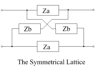
Lattice delay networks are an important subgroup of lattice networks. They are all-pass filters, so they have a flat amplitude response, but a phase response which varies linearly with frequency. All lattice circuits, regardless of their complexity, are based on the schematic shown below, which contains two series impedances, Za, and two shunt impedances, Zb. Although there is duplication of impedances in this arrangement, it offers great flexibility to the circuit designer so that, in addition to its use as delay network it can be configured to be a phase corrector, a dispersive network, an amplitude equalizer, or a low pass filter, according to the choice of components for the lattice elements.
References
↑ Daniels, Richard W. (1974). Approximation Methods for Electronic Filter Design. New York: McGraw-Hill. ISBN0-07-015308-6.
↑ Matthaei, George L.; Young, Leo; Jones, E. M. T. (1980). Microwave Filters, Impedance-Matching Networks, and Coupling Structures. Norwood, MA: Artech House. ISBN0-89-006099-1.
This page is based on this Wikipedia article Text is available under the CC BY-SA 4.0 license; additional terms may apply. Images, videos and audio are available under their respective licenses.