In statistics, a normal distribution or Gaussian distribution is a type of continuous probability distribution for a real-valued random variable. The general form of its probability density function is
In probability and statistics, an exponential family is a parametric set of probability distributions of a certain form, specified below. This special form is chosen for mathematical convenience, including the enabling of the user to calculate expectations, covariances using differentiation based on some useful algebraic properties, as well as for generality, as exponential families are in a sense very natural sets of distributions to consider. The term exponential class is sometimes used in place of "exponential family", or the older term Koopman–Darmois family. Sometimes loosely referred to as "the" exponential family, this class of distributions is distinct because they all possess a variety of desirable properties, most importantly the existence of a sufficient statistic.
In physics and astronomy, the Reissner–Nordström metric is a static solution to the Einstein–Maxwell field equations, which corresponds to the gravitational field of a charged, non-rotating, spherically symmetric body of mass M. The analogous solution for a charged, rotating body is given by the Kerr–Newman metric.
In probability theory, a Lévy process, named after the French mathematician Paul Lévy, is a stochastic process with independent, stationary increments: it represents the motion of a point whose successive displacements are random, in which displacements in pairwise disjoint time intervals are independent, and displacements in different time intervals of the same length have identical probability distributions. A Lévy process may thus be viewed as the continuous-time analog of a random walk.
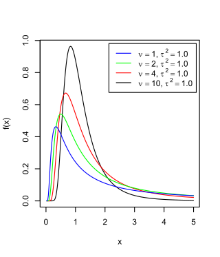
The scaled inverse chi-squared distribution is the distribution for x = 1/s2, where s2 is a sample mean of the squares of ν independent normal random variables that have mean 0 and inverse variance 1/σ2 = τ2. The distribution is therefore parametrised by the two quantities ν and τ2, referred to as the number of chi-squared degrees of freedom and the scaling parameter, respectively.
In Bayesian statistics, a maximum a posteriori probability (MAP) estimate is an estimate of an unknown quantity, that equals the mode of the posterior distribution. The MAP can be used to obtain a point estimate of an unobserved quantity on the basis of empirical data. It is closely related to the method of maximum likelihood (ML) estimation, but employs an augmented optimization objective which incorporates a prior distribution over the quantity one wants to estimate. MAP estimation can therefore be seen as a regularization of maximum likelihood estimation.
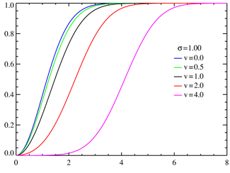
The noncentral t-distribution generalizes Student's t-distribution using a noncentrality parameter. Whereas the central probability distribution describes how a test statistic t is distributed when the difference tested is null, the noncentral distribution describes how t is distributed when the null is false. This leads to its use in statistics, especially calculating statistical power. The noncentral t-distribution is also known as the singly noncentral t-distribution, and in addition to its primary use in statistical inference, is also used in robust modeling for data.
Ellipsoidal coordinates are a three-dimensional orthogonal coordinate system that generalizes the two-dimensional elliptic coordinate system. Unlike most three-dimensional orthogonal coordinate systems that feature quadratic coordinate surfaces, the ellipsoidal coordinate system is based on confocal quadrics.
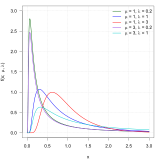
In probability theory, the inverse Gaussian distribution is a two-parameter family of continuous probability distributions with support on (0,∞).
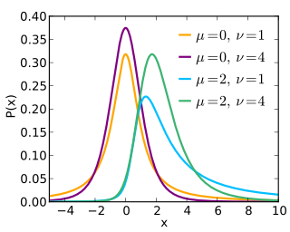
In statistics, the multivariate t-distribution is a multivariate probability distribution. It is a generalization to random vectors of the Student's t-distribution, which is a distribution applicable to univariate random variables. While the case of a random matrix could be treated within this structure, the matrix t-distribution is distinct and makes particular use of the matrix structure.
Expected shortfall (ES) is a risk measure—a concept used in the field of financial risk measurement to evaluate the market risk or credit risk of a portfolio. The "expected shortfall at q% level" is the expected return on the portfolio in the worst of cases. ES is an alternative to value at risk that is more sensitive to the shape of the tail of the loss distribution.
A ratio distribution is a probability distribution constructed as the distribution of the ratio of random variables having two other known distributions. Given two random variables X and Y, the distribution of the random variable Z that is formed as the ratio Z = X/Y is a ratio distribution.

In probability theory and statistics, the half-normal distribution is a special case of the folded normal distribution.

In probability theory and statistics, the normal-inverse-gamma distribution is a four-parameter family of multivariate continuous probability distributions. It is the conjugate prior of a normal distribution with unknown mean and variance.

In probability theory and directional statistics, a wrapped normal distribution is a wrapped probability distribution that results from the "wrapping" of the normal distribution around the unit circle. It finds application in the theory of Brownian motion and is a solution to the heat equation for periodic boundary conditions. It is closely approximated by the von Mises distribution, which, due to its mathematical simplicity and tractability, is the most commonly used distribution in directional statistics.
In statistics, identifiability is a property which a model must satisfy for precise inference to be possible. A model is identifiable if it is theoretically possible to learn the true values of this model's underlying parameters after obtaining an infinite number of observations from it. Mathematically, this is equivalent to saying that different values of the parameters must generate different probability distributions of the observable variables. Usually the model is identifiable only under certain technical restrictions, in which case the set of these requirements is called the identification conditions.
In statistics, an adaptive estimator is an estimator in a parametric or semiparametric model with nuisance parameters such that the presence of these nuisance parameters does not affect efficiency of estimation.
In statistics and probability theory, the nonparametric skew is a statistic occasionally used with random variables that take real values. It is a measure of the skewness of a random variable's distribution—that is, the distribution's tendency to "lean" to one side or the other of the mean. Its calculation does not require any knowledge of the form of the underlying distribution—hence the name nonparametric. It has some desirable properties: it is zero for any symmetric distribution; it is unaffected by a scale shift; and it reveals either left- or right-skewness equally well. In some statistical samples it has been shown to be less powerful than the usual measures of skewness in detecting departures of the population from normality.
In statistics, the variance function is a smooth function that depicts the variance of a random quantity as a function of its mean. The variance function is a measure of heteroscedasticity and plays a large role in many settings of statistical modelling. It is a main ingredient in the generalized linear model framework and a tool used in non-parametric regression, semiparametric regression and functional data analysis. In parametric modeling, variance functions take on a parametric form and explicitly describe the relationship between the variance and the mean of a random quantity. In a non-parametric setting, the variance function is assumed to be a smooth function.

In probability theory, the stable count distribution is the conjugate prior of a one-sided stable distribution. This distribution was discovered by Stephen Lihn in his 2017 study of daily distributions of the S&P 500 and the VIX. The stable distribution family is also sometimes referred to as the Lévy alpha-stable distribution, after Paul Lévy, the first mathematician to have studied it.