Confluent hypergeometric function

Last updated November 03, 2023

In mathematics, a confluent hypergeometric function is a solution of a confluent hypergeometric equation, which is a degenerate form of a hypergeometric differential equation where two of the three regular singularities merge into an irregular singularity. The term confluent refers to the merging of singular points of families of differential equations; confluere is Latin for "to flow together". There are several common standard forms of confluent hypergeometric functions:

Kummer's (confluent hypergeometric) function $M (a, b, z)$ , introduced by Kummer ( 1837 ), is a solution to Kummer's differential equation. This is also known as the confluent hypergeometric function of the first kind. There is a different and unrelated Kummer's function bearing the same name.
Tricomi's (confluent hypergeometric) function $U (a, b, z)$ introduced by FrancescoTricomi ( 1947 ), sometimes denoted by $Ψ(a; b; z)$ , is another solution to Kummer's equation. This is also known as the confluent hypergeometric function of the second kind.
Whittaker functions (for Edmund Taylor Whittaker) are solutions to Whittaker's equation.
Coulomb wave functions are solutions to the Coulomb wave equation.

The Kummer functions, Whittaker functions, and Coulomb wave functions are essentially the same, and differ from each other only by elementary functions and change of variables.

Kummer's equation

Kummer's equation may be written as:

z{\frac {d^{2}w}{dz^{2}}}+(b-z){\frac {dw}{dz}}-aw=0,

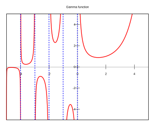
with a regular singular point at $z = 0$ and an irregular singular point at $z = \infty$ . It has two (usually) linearly independent solutions $M (a, b, z)$ and $U (a, b, z)$ .

Kummer's function of the first kind $M$ is a generalized hypergeometric series introduced in ( Kummer 1837 ), given by:

M(a,b,z)=\sum _{n=0}^{\infty }{\frac {a^{(n)}z^{n}}{b^{(n)}n!}}={}_{1}F_{1}(a;b;z),

where:

a^{(0)}=1,

a^{(n)}=a(a+1)(a+2)\cdots (a+n-1)\,,

is the rising factorial. Another common notation for this solution is $Φ(a, b, z)$ . Considered as a function of $a$ , $b$ , or $z$ with the other two held constant, this defines an entire function of $a$ or $z$ , except when $b = 0, -1, -2, ...$ As a function of $b$ it is analytic except for poles at the non-positive integers.

Some values of $a$ and $b$ yield solutions that can be expressed in terms of other known functions. See #Special cases. When $a$ is a non-positive integer, then Kummer's function (if it is defined) is a generalized Laguerre polynomial.

Just as the confluent differential equation is a limit of the hypergeometric differential equation as the singular point at 1 is moved towards the singular point at ∞, the confluent hypergeometric function can be given as a limit of the hypergeometric function

M(a,c,z)=\lim _{b\to \infty }{}_{2}F_{1}(a,b;c;z/b)

and many of the properties of the confluent hypergeometric function are limiting cases of properties of the hypergeometric function.

Since Kummer's equation is second order there must be another, independent, solution. The indicial equation of the method of Frobenius tells us that the lowest power of a power series solution to the Kummer equation is either 0 or $1 - b$ . If we let $w (z)$ be

w(z)=z^{1-b}v(z)

then the differential equation gives

z^{2-b}{\frac {d^{2}v}{dz^{2}}}+2(1-b)z^{1-b}{\frac {dv}{dz}}-b(1-b)z^{-b}v+(b-z)\left[z^{1-b}{\frac {dv}{dz}}+(1-b)z^{-b}v\right]-az^{1-b}v=0

which, upon dividing out $z 1- b$ and simplifying, becomes

z{\frac {d^{2}v}{dz^{2}}}+(2-b-z){\frac {dv}{dz}}-(a+1-b)v=0.

This means that $z 1- b M (a + 1 - b, 2 - b, z)$ is a solution so long as $b$ is not an integer greater than 1, just as $M (a, b, z)$ is a solution so long as $b$ is not an integer less than 1. We can also use the Tricomi confluent hypergeometric function $U (a, b, z)$ introduced by FrancescoTricomi ( 1947 ), and sometimes denoted by $Ψ(a; b; z)$ . It is a combination of the above two solutions, defined by

U(a,b,z)={\frac {\Gamma (1-b)}{\Gamma (a+1-b)}}M(a,b,z)+{\frac {\Gamma (b-1)}{\Gamma (a)}}z^{1-b}M(a+1-b,2-b,z).

Although this expression is undefined for integer $b$ , it has the advantage that it can be extended to any integer $b$ by continuity. Unlike Kummer's function which is an entire function of $z$ , $U (z)$ usually has a singularity at zero. For example, if $b = 0$ and $a \neq 0$ then $Γ(a +1) U (a, b, z) - 1$ is asymptotic to $az ln z$ as $z$ goes to zero. But see #Special cases for some examples where it is an entire function (polynomial).

Note that the solution $z 1- b U (a + 1 - b, 2 - b, z)$ to Kummer's equation is the same as the solution $U (a, b, z)$ , see #Kummer's transformation.

For most combinations of real or complex $a$ and $b$ , the functions $M (a, b, z)$ and $U (a, b, z)$ are independent, and if $b$ is a non-positive integer, so $M (a, b, z)$ doesn't exist, then we may be able to use $z 1- b M (a +1- b, 2- b, z)$ as a second solution. But if $a$ is a non-positive integer and $b$ is not a non-positive integer, then $U (z)$ is a multiple of $M (z)$ . In that case as well, $z 1- b M (a +1- b, 2- b, z)$ can be used as a second solution if it exists and is different. But when $b$ is an integer greater than 1, this solution doesn't exist, and if $b = 1$ then it exists but is a multiple of $U (a, b, z)$ and of $M (a, b, z)$ In those cases a second solution exists of the following form and is valid for any real or complex $a$ and any positive integer $b$ except when $a$ is a positive integer less than $b$ :

M(a,b,z)\ln z+z^{1-b}\sum _{k=0}^{\infty }C_{k}z^{k}

When a = 0 we can alternatively use:

\int _{-\infty }^{z}(-u)^{-b}e^{u}\mathrm {d} u.

When $b = 1$ this is the exponential integral $E 1 (-z)$ .

A similar problem occurs when $a - b$ is a negative integer and $b$ is an integer less than 1. In this case $M (a, b, z)$ doesn't exist, and $U (a, b, z)$ is a multiple of $z 1- b M (a +1- b, 2- b, z).$ A second solution is then of the form:

z^{1-b}M(a+1-b,2-b,z)\ln z+\sum _{k=0}^{\infty }C_{k}z^{k}

Other equations

Confluent Hypergeometric Functions can be used to solve the Extended Confluent Hypergeometric Equation whose general form is given as:

z{\frac {d^{2}w}{dz^{2}}}+(b-z){\frac {dw}{dz}}-\left(\sum _{m=0}^{M}a_{m}z^{m}\right)w=0

^[1]

Note that for $M = 0$ or when the summation involves just one term, it reduces to the conventional Confluent Hypergeometric Equation.

Thus Confluent Hypergeometric Functions can be used to solve "most" second-order ordinary differential equations whose variable coefficients are all linear functions of $z$ , because they can be transformed to the Extended Confluent Hypergeometric Equation. Consider the equation:

(A+Bz){\frac {d^{2}w}{dz^{2}}}+(C+Dz){\frac {dw}{dz}}+(E+Fz)w=0

First we move the regular singular point to $0$ by using the substitution of $A + Bz \mapsto z$ , which converts the equation to:

z{\frac {d^{2}w}{dz^{2}}}+(C+Dz){\frac {dw}{dz}}+(E+Fz)w=0

with new values of $C, D, E$ , and $F$ . Next we use the substitution:

z\mapsto {\frac {1}{\sqrt {D^{2}-4F}}}z

and multiply the equation by the same factor, obtaining:

z{\frac {d^{2}w}{dz^{2}}}+\left(C+{\frac {D}{\sqrt {D^{2}-4F}}}z\right){\frac {dw}{dz}}+\left({\frac {E}{\sqrt {D^{2}-4F}}}+{\frac {F}{D^{2}-4F}}z\right)w=0

whose solution is

\exp \left(-\left(1+{\frac {D}{\sqrt {D^{2}-4F}}}\right){\frac {z}{2}}\right)w(z),

where $w (z)$ is a solution to Kummer's equation with

a=\left(1+{\frac {D}{\sqrt {D^{2}-4F}}}\right){\frac {C}{2}}-{\frac {E}{\sqrt {D^{2}-4F}}},\qquad b=C.

Note that the square root may give an imaginary or complex number. If it is zero, another solution must be used, namely

\exp \left(-{\tfrac {1}{2}}Dz\right)w(z),

where $w (z)$ is a confluent hypergeometric limit function satisfying

zw''(z)+Cw'(z)+\left(E-{\tfrac {1}{2}}CD\right)w(z)=0.

As noted below, even the Bessel equation can be solved using confluent hypergeometric functions.

Integral representations

If $Re b > Re a > 0$ , $M (a, b, z)$ can be represented as an integral

M(a,b,z)={\frac {\Gamma (b)}{\Gamma (a)\Gamma (b-a)}}\int _{0}^{1}e^{zu}u^{a-1}(1-u)^{b-a-1}\,du.

thus $M (a, a + b, it)$ is the characteristic function of the beta distribution. For $a$ with positive real part $U$ can be obtained by the Laplace integral

U(a,b,z)={\frac {1}{\Gamma (a)}}\int _{0}^{\infty }e^{-zt}t^{a-1}(1+t)^{b-a-1}\,dt,\quad (\operatorname {Re} \ a>0)

The integral defines a solution in the right half-plane $Re z > 0$ .

They can also be represented as Barnes integrals

M(a,b,z)={\frac {1}{2\pi i}}{\frac {\Gamma (b)}{\Gamma (a)}}\int _{-i\infty }^{i\infty }{\frac {\Gamma (-s)\Gamma (a+s)}{\Gamma (b+s)}}(-z)^{s}ds

where the contour passes to one side of the poles of $Γ(- s)$ and to the other side of the poles of $Γ(a + s)$ .

Asymptotic behavior

If a solution to Kummer's equation is asymptotic to a power of $z$ as $z \to \infty$ , then the power must be $- a$ . This is in fact the case for Tricomi's solution $U (a, b, z)$ . Its asymptotic behavior as $z \to \infty$ can be deduced from the integral representations. If $z = x \in R$ , then making a change of variables in the integral followed by expanding the binomial series and integrating it formally term by term gives rise to an asymptotic series expansion, valid as $x \to \infty$ :^[2]

U(a,b,x)\sim x^{-a}\,_{2}F_{0}\left(a,a-b+1;\,;-{\frac {1}{x}}\right),

where ${\displaystyle _{2}F_{0}(\cdot ,\cdot$ is a generalized hypergeometric series with 1 as leading term, which generally converges nowhere, but exists as a formal power series in $1/ x$ . This asymptotic expansion is also valid for complex $z$ instead of real $x$ , with $| arg z | < 3 π /2.$

The asymptotic behavior of Kummer's solution for large $| z |$ is:

M(a,b,z)\sim \Gamma (b)\left({\frac {e^{z}z^{a-b}}{\Gamma (a)}}+{\frac {(-z)^{-a}}{\Gamma (b-a)}}\right)

The powers of $z$ are taken using $-3 π /2 < arg z \leq π /2$ .^[3] The first term is not needed when $Γ(b - a)$ is finite, that is when $b - a$ is not a non-positive integer and the real part of $z$ goes to negative infinity, whereas the second term is not needed when $Γ(a)$ is finite, that is, when $a$ is a not a non-positive integer and the real part of $z$ goes to positive infinity.

There is always some solution to Kummer's equation asymptotic to $e z z a - b$ as $z \to -\infty$ . Usually this will be a combination of both $M (a, b, z)$ and $U (a, b, z)$ but can also be expressed as $e z (-1) a - b U (b - a, b, - z)$ .

Relations

There are many relations between Kummer functions for various arguments and their derivatives. This section gives a few typical examples.

Contiguous relations

Given $M (a, b, z)$ , the four functions $M (a \pm 1, b, z), M (a, b \pm 1, z)$ are called contiguous to $M (a, b, z)$ . The function $M (a, b, z)$ can be written as a linear combination of any two of its contiguous functions, with rational coefficients in terms of $a, b$ , and $z$ . This gives $(42) = 6$ relations, given by identifying any two lines on the right hand side of

{\begin{aligned}z{\frac {dM}{dz}}=z{\frac {a}{b}}M(a+,b+)&=a(M(a+)-M)\\&=(b-1)(M(b-)-M)\\&=(b-a)M(a-)+(a-b+z)M\\&=z(a-b)M(b+)/b+zM\\\end{aligned}}

In the notation above, $M = M (a, b, z)$ , $M (a +) = M (a + 1, b, z)$ , and so on.

Repeatedly applying these relations gives a linear relation between any three functions of the form $M (a + m, b + n, z)$ (and their higher derivatives), where $m$ , $n$ are integers.

There are similar relations for $U$ .

Kummer's transformation

Kummer's functions are also related by Kummer's transformations:

M(a,b,z)=e^{z}\,M(b-a,b,-z)

U(a,b,z)=z^{1-b}U\left(1+a-b,2-b,z\right)

.

Multiplication theorem

The following multiplication theorems hold true:

{\begin{aligned}U(a,b,z)&=e^{(1-t)z}\sum _{i=0}{\frac {(t-1)^{i}z^{i}}{i!}}U(a,b+i,zt)\\&=e^{(1-t)z}t^{b-1}\sum _{i=0}{\frac {\left(1-{\frac {1}{t}}\right)^{i}}{i!}}U(a-i,b-i,zt).\end{aligned}}

Connection with Laguerre polynomials and similar representations

In terms of Laguerre polynomials, Kummer's functions have several expansions, for example

M\left(a,b,{\frac {xy}{x-1}}\right)=(1-x)^{a}\cdot \sum _{n}{\frac {a^{(n)}}{b^{(n)}}}L_{n}^{(b-1)}(y)x^{n}

( Erdélyi et al. 1953 , 6.12)

or

\operatorname {M} \left(a;\,b;\,z\right)={\frac {\Gamma \left(1-a\right)\cdot \Gamma \left(b\right)}{\Gamma \left(b-a\right)}}\cdot \operatorname {L_{-a}^{b-1}} \left(z\right)

Special cases

Functions that can be expressed as special cases of the confluent hypergeometric function include:

Some elementary functions where the left-hand side is not defined when $b$ is a non-positive integer, but the right-hand side is still a solution of the corresponding Kummer equation:

M(0,b,z)=1

U(0,c,z)=1

M(b,b,z)=e^{z}

U(a,a,z)=e^{z}\int _{z}^{\infty }u^{-a}e^{-u}du

(a polynomial if

a

is a non-positive integer)

{\frac {U(1,b,z)}{\Gamma (b-1)}}+{\frac {M(1,b,z)}{\Gamma (b)}}=z^{1-b}e^{z}

M(n,b,z)

for non-positive integer

n

is a generalized Laguerre polynomial.

U(n,c,z)

for non-positive integer

n

is a multiple of a generalized Laguerre polynomial, equal to

{\tfrac {\Gamma (1-c)}{\Gamma (n+1-c)}}M(n,c,z)

when the latter exists.

U(c-n,c,z)

when

n

is a positive integer is a closed form with powers of

z

, equal to

{\tfrac {\Gamma (c-1)}{\Gamma (c-n)}}z^{1-c}M(1-n,2-c,z)

when the latter exists.

U(a,a+1,z)=z^{-a}

U(-n,-2n,z)

for non-negative integer

n

is a Bessel polynomial (see lower down).

M(1,2,z)=(e^{z}-1)/z,\ \ M(1,3,z)=2!(e^{z}-1-z)/z^{2}

etc.

Using the contiguous relation

aM(a+)=(a+z)M+z(a-b)M(b+)/b

we get, for example,

M(2,1,z)=(1+z)e^{z}.

Bateman's function
Bessel functions and many related functions such as Airy functions, Kelvin functions, Hankel functions. For example, in the special case $b = 2 a$ the function reduces to a Bessel function:

{}_{1}F_{1}(a,2a,x)=e^{x/2}\,{}_{0}F_{1}\left(;a+{\tfrac {1}{2}};{\tfrac {x^{2}}{16}}\right)=e^{x/2}\left({\tfrac {x}{4}}\right)^{1/2-a}\Gamma \left(a+{\tfrac {1}{2}}\right)I_{a-1/2}\left({\tfrac {x}{2}}\right).

This identity is sometimes also referred to as Kummer's second transformation. Similarly

U(a,2a,x)={\frac {e^{x/2}}{\sqrt {\pi }}}x^{1/2-a}K_{a-1/2}(x/2),

When

a

is a non-positive integer, this equals

2 - a θ - a (x /2)

where

θ

is a Bessel polynomial.

The error function can be expressed as

\mathrm {erf} (x)={\frac {2}{\sqrt {\pi }}}\int _{0}^{x}e^{-t^{2}}dt={\frac {2x}{\sqrt {\pi }}}\ {}_{1}F_{1}\left({\tfrac {1}{2}},{\tfrac {3}{2}},-x^{2}\right).

Coulomb wave function
Cunningham functions
Exponential integral and related functions such as the sine integral, logarithmic integral
Hermite polynomials
Incomplete gamma function
Laguerre polynomials
Parabolic cylinder function (or Weber function)
Poisson–Charlier function
Toronto functions
Whittaker functions $M κ,μ (z), W κ,μ (z)$ are solutions of Whittaker's equation that can be expressed in terms of Kummer functions $M$ and $U$ by

M_{\kappa ,\mu }(z)=e^{-{\tfrac {z}{2}}}z^{\mu +{\tfrac {1}{2}}}M\left(\mu -\kappa +{\tfrac {1}{2}},1+2\mu ;z\right)

W_{\kappa ,\mu }(z)=e^{-{\tfrac {z}{2}}}z^{\mu +{\tfrac {1}{2}}}U\left(\mu -\kappa +{\tfrac {1}{2}},1+2\mu ;z\right)

The general $p$ -th raw moment ( $p$ not necessarily an integer) can be expressed as^[4]

{\begin{aligned}\operatorname {E} \left[\left|N\left(\mu ,\sigma ^{2}\right)\right|^{p}\right]&={\frac {\left(2\sigma ^{2}\right)^{p/2}\Gamma \left({\tfrac {1+p}{2}}\right)}{\sqrt {\pi }}}\ {}_{1}F_{1}\left(-{\tfrac {p}{2}},{\tfrac {1}{2}},-{\tfrac {\mu ^{2}}{2\sigma ^{2}}}\right)\\\operatorname {E} \left[N\left(\mu ,\sigma ^{2}\right)^{p}\right]&=\left(-2\sigma ^{2}\right)^{p/2}U\left(-{\tfrac {p}{2}},{\tfrac {1}{2}},-{\tfrac {\mu ^{2}}{2\sigma ^{2}}}\right)\end{aligned}}

In the second formula the function's second branch cut can be chosen by multiplying with

(-1) p

.

Application to continued fractions

By applying a limiting argument to Gauss's continued fraction it can be shown that

{\frac {M(a+1,b+1,z)}{M(a,b,z)}}={\cfrac {1}{1-{\cfrac {\displaystyle {\frac {b-a}{b(b+1)}}z}{1+{\cfrac {\displaystyle {\frac {a+1}{(b+1)(b+2)}}z}{1-{\cfrac {\displaystyle {\frac {b-a+1}{(b+2)(b+3)}}z}{1+{\cfrac {\displaystyle {\frac {a+2}{(b+3)(b+4)}}z}{1-\ddots }}}}}}}}}}

and that this continued fraction converges uniformly to a meromorphic function of $z$ in every bounded domain that does not include a pole.

Notes

↑ Campos, LMBC (2001). "On Some Solutions of the Extended Confluent Hypergeometric Differential Equation". Journal of Computational and Applied Mathematics. Elsevier. 137: 177–200. doi: 10.1016/s0377-0427(00)00706-8 .
↑ Andrews, G.E.; Askey, R.; Roy, R. (2001). Special functions. Cambridge University Press. ISBN 978-0521789882..
↑ This is derived from Abramowitz and Stegun (see reference below), page 508, where a full asymptotic series is given. They switch the sign of the exponent in $exp(iπa)$ in the right half-plane but this is immaterial, as the term is negligible there or else $a$ is an integer and the sign doesn't matter.
↑ "Aspects of Multivariate Statistical Theory | Wiley". Wiley.com. Retrieved 2021-01-23.

Related Research Articles

Bessel functions, first defined by the mathematician Daniel Bernoulli and then generalized by Friedrich Bessel, are canonical solutions $y (x)$ of Bessel's differential equation

In mathematics, the gamma function is one commonly used extension of the factorial function to complex numbers. The gamma function is defined for all complex numbers except the non-positive integers. For every positive integer $n$ ,

In mathematics, the Lambert $W$ function, also called the omega function or product logarithm, is a multivalued function, namely the branches of the converse relation of the function $f (w) = we w$ , where $w$ is any complex number and $e w$ is the exponential function.

In physical science and mathematics, the Legendre functions $P λ$ , $Q λ$ and associated Legendre functions $P μ λ$ , $Q μ λ$ , and Legendre functions of the second kind, $Q n$ , are all solutions of Legendre's differential equation. The Legendre polynomials and the associated Legendre polynomials are also solutions of the differential equation in special cases, which, by virtue of being polynomials, have a large number of additional properties, mathematical structure, and applications. For these polynomial solutions, see the separate Wikipedia articles.

In mathematics, a generalized hypergeometric series is a power series in which the ratio of successive coefficients indexed by n is a rational function of n. The series, if convergent, defines a generalized hypergeometric function, which may then be defined over a wider domain of the argument by analytic continuation. The generalized hypergeometric series is sometimes just called the hypergeometric series, though this term also sometimes just refers to the Gaussian hypergeometric series. Generalized hypergeometric functions include the (Gaussian) hypergeometric function and the confluent hypergeometric function as special cases, which in turn have many particular special functions as special cases, such as elementary functions, Bessel functions, and the classical orthogonal polynomials.

In mathematics, the upper and lower incomplete gamma functions are types of special functions which arise as solutions to various mathematical problems such as certain integrals.

In mathematics, the exponential integral Ei is a special function on the complex plane.

In mathematics, the associated Legendre polynomials are the canonical solutions of the general Legendre equation

In mathematics, the parabolic cylinder functions are special functions defined as solutions to the differential equation

In probability theory and statistics, the chi distribution is a continuous probability distribution over the non-negative real line. It is the distribution of the positive square root of a sum of squared independent Gaussian random variables. Equivalently, it is the distribution of the Euclidean distance between a multivariate Gaussian random variable and the origin. It is thus related to the chi-squared distribution by describing the distribution of the positive square roots of a variable obeying a chi-squared distribution.

In mathematics, the Gaussian or ordinary hypergeometric function₂F₁(a,b;c;z) is a special function represented by the hypergeometric series, that includes many other special functions as specific or limiting cases. It is a solution of a second-order linear ordinary differential equation (ODE). Every second-order linear ODE with three regular singular points can be transformed into this equation.

In mathematics, the local Heun function $is the solution of Heun's differential equation that is holomorphic and 1 at the singular point z = 0. The local Heun function is called a Heun function, denoted Hf, if it is also regular at z = 1, and is called a Heun polynomial, denoted Hp, if it is regular at all three finite singular points z = 0, 1, a .$

In mathematics, Riemann's differential equation, named after Bernhard Riemann, is a generalization of the hypergeometric differential equation, allowing the regular singular points to occur anywhere on the Riemann sphere, rather than merely at 0, 1, and $. The equation is also known as the Papperitz equation .$

In mathematics, a Whittaker function is a special solution of Whittaker's equation, a modified form of the confluent hypergeometric equation introduced by Whittaker (1903) to make the formulas involving the solutions more symmetric. More generally, Jacquet (1966, 1967) introduced Whittaker functions of reductive groups over local fields, where the functions studied by Whittaker are essentially the case where the local field is the real numbers and the group is SL₂(R).

<span class="mw-page-title-main">ARGUS distribution</span>

In physics, the ARGUS distribution, named after the particle physics experiment ARGUS, is the probability distribution of the reconstructed invariant mass of a decayed particle candidate in continuum background.

In mathematics, the G-function was introduced by Cornelis Simon Meijer (1936) as a very general function intended to include most of the known special functions as particular cases. This was not the only attempt of its kind: the generalized hypergeometric function and the MacRobert E-function had the same aim, but Meijer's G-function was able to include those as particular cases as well. The first definition was made by Meijer using a series; nowadays the accepted and more general definition is via a line integral in the complex plane, introduced in its full generality by Arthur Erdélyi in 1953.

A hydrogen-like atom (or hydrogenic atom) is any atom or ion with a single valence electron. These atoms are isoelectronic with hydrogen. Examples of hydrogen-like atoms include, but are not limited to, hydrogen itself, all alkali metals such as Rb and Cs, singly ionized alkaline earth metals such as Ca⁺ and Sr⁺ and other ions such as He⁺, Li²⁺, and Be³⁺ and isotopes of any of the above. A hydrogen-like atom includes a positively charged core consisting of the atomic nucleus and any core electrons as well as a single valence electron. Because helium is common in the universe, the spectroscopy of singly ionized helium is important in EUV astronomy, for example, of DO white dwarf stars.

In mathematics, the Struve functions $H α (x)$ , are solutions $y (x)$ of the non-homogeneous Bessel's differential equation:

In mathematics, Jacobi polynomials $are a class of classical orthogonal polynomials. They are orthogonal with respect to the weight on the interval . The Gegenbauer polynomials, and thus also the Legendre, Zernike and Chebyshev polynomials, are special cases of the Jacobi polynomials.$

In mathematics, the sinhc function appears frequently in papers about optical scattering, Heisenberg spacetime and hyperbolic geometry. For $, it is defined as$

References

Abramowitz, Milton; Stegun, Irene Ann, eds. (1983) [June 1964]. "Chapter 13". Handbook of Mathematical Functions with Formulas, Graphs, and Mathematical Tables. Applied Mathematics Series. Vol. 55 (Ninth reprint with additional corrections of tenth original printing with corrections (December 1972); first ed.). Washington D.C.; New York: United States Department of Commerce, National Bureau of Standards; Dover Publications. p. 504. ISBN 978-0-486-61272-0. LCCN 64-60036. MR 0167642. LCCN 65-12253.
Chistova, E.A. (2001) [1994], "Confluent hypergeometric function", Encyclopedia of Mathematics , EMS Press
Daalhuis, Adri B. Olde (2010), "Confluent hypergeometric function", in Olver, Frank W. J.; Lozier, Daniel M.; Boisvert, Ronald F.; Clark, Charles W. (eds.), NIST Handbook of Mathematical Functions , Cambridge University Press, ISBN 978-0-521-19225-5, MR 2723248 .
Erdélyi, Arthur; Magnus, Wilhelm; Oberhettinger, Fritz & Tricomi, Francesco G. (1953). Higher transcendental functions. Vol. I. New York–Toronto–London: McGraw–Hill Book Company, Inc. MR 0058756.
Kummer, Ernst Eduard (1837). "De integralibus quibusdam definitis et seriebus infinitis". Journal für die reine und angewandte Mathematik (in Latin). 1837 (17): 228–242. doi:10.1515/crll.1837.17.228. ISSN 0075-4102. S2CID 121351583.
Slater, Lucy Joan (1960). Confluent hypergeometric functions . Cambridge, UK: Cambridge University Press. MR 0107026.
Tricomi, Francesco G. (1947). "Sulle funzioni ipergeometriche confluenti". Annali di Matematica Pura ed Applicata. Series 4 (in Italian). 26: 141–175. doi: 10.1007/bf02415375 . ISSN 0003-4622. MR 0029451. S2CID 119860549.
Tricomi, Francesco G. (1954). Funzioni ipergeometriche confluenti. Consiglio Nazionale Delle Ricerche Monografie Matematiche (in Italian). Vol. 1. Rome: Edizioni cremonese. ISBN 978-88-7083-449-9. MR 0076936.
Oldham, K.B.; Myland, J.; Spanier, J. (2010). An Atlas of Functions: with Equator, the Atlas Function Calculator. An Atlas of Functions. Springer New York. ISBN 978-0-387-48807-3 . Retrieved 2017-08-23.

External links

Confluent Hypergeometric Functions in NIST Digital Library of Mathematical Functions
Kummer hypergeometric function on the Wolfram Functions site
Tricomi hypergeometric function on the Wolfram Functions site

This page is based on this Wikipedia article
Text is available under the CC BY-SA 4.0 license; additional terms may apply.
Images, videos and audio are available under their respective licenses.

[1] Campos, LMBC (2001). "On Some Solutions of the Extended Confluent Hypergeometric Differential Equation". Journal of Computational and Applied Mathematics. Elsevier. 137: 177–200. doi: 10.1016/s0377-0427(00)00706-8 .

[2] Andrews, G.E.; Askey, R.; Roy, R. (2001). Special functions. Cambridge University Press. ISBN 978-0521789882..

[3] This is derived from Abramowitz and Stegun (see reference below), page 508, where a full asymptotic series is given. They switch the sign of the exponent in $exp(iπa)$ in the right half-plane but this is immaterial, as the term is negligible there or else $a$ is an integer and the sign doesn't matter.

[4] "Aspects of Multivariate Statistical Theory | Wiley". Wiley.com. Retrieved 2021-01-23.

[1]

[2]

[3]

[4]