Bellman equation

Last updated
Bellman flow chart Bellman flow chart.png
Bellman flow chart

A Bellman equation, named after Richard E. Bellman, is a necessary condition for optimality associated with the mathematical optimization method known as dynamic programming. [1] It writes the "value" of a decision problem at a certain point in time in terms of the payoff from some initial choices and the "value" of the remaining decision problem that results from those initial choices. [2] This breaks a dynamic optimization problem into a sequence of simpler subproblems, as Bellman's “principle of optimality" prescribes. [3] The equation applies to algebraic structures with a total ordering; for algebraic structures with a partial ordering, the generic Bellman's equation can be used. [4]

Contents

The Bellman equation was first applied to engineering control theory and to other topics in applied mathematics, and subsequently became an important tool in economic theory; though the basic concepts of dynamic programming are prefigured in John von Neumann and Oskar Morgenstern's Theory of Games and Economic Behavior and Abraham Wald's sequential analysis .[ citation needed ] The term 'Bellman equation' usually refers to the dynamic programming equation associated with discrete-time optimization problems. [5] In continuous-time optimization problems, the analogous equation is a partial differential equation that is called the Hamilton–Jacobi–Bellman equation. [6] [7]

In discrete time any multi-stage optimization problem can be solved by analyzing the appropriate Bellman equation. The appropriate Bellman equation can be found by introducing new state variables (state augmentation). [8] However, the resulting augmented-state multi-stage optimization problem has a higher dimensional state space than the original multi-stage optimization problem - an issue that can potentially render the augmented problem intractable due to the “curse of dimensionality”. Alternatively, it has been shown that if the cost function of the multi-stage optimization problem satisfies a "backward separable" structure, then the appropriate Bellman equation can be found without state augmentation. [9]

Analytical concepts in dynamic programming

To understand the Bellman equation, several underlying concepts must be understood. First, any optimization problem has some objective: minimizing travel time, minimizing cost, maximizing profits, maximizing utility, etc. The mathematical function that describes this objective is called the objective function .[ citation needed ]

Dynamic programming breaks a multi-period planning problem into simpler steps at different points in time. Therefore, it requires keeping track of how the decision situation is evolving over time. The information about the current situation that is needed to make a correct decision is called the "state". [10] [11] For example, to decide how much to consume and spend at each point in time, people would need to know (among other things) their initial wealth. Therefore, wealth would be one of their state variables , but there would probably be others.[ citation needed ]

The variables chosen at any given point in time are often called the control variables . For instance, given their current wealth, people might decide how much to consume now. Choosing the control variables now may be equivalent to choosing the next state; more generally, the next state is affected by other factors in addition to the current control. For example, in the simplest case, today's wealth (the state) and consumption (the control) might exactly determine tomorrow's wealth (the new state), though typically other factors will affect tomorrow's wealth too.[ citation needed ]

The dynamic programming approach describes the optimal plan by finding a rule that tells what the controls should be, given any possible value of the state. For example, if consumption (c) depends only on wealth (W), we would seek a rule that gives consumption as a function of wealth. Such a rule, determining the controls as a function of the states, is called a policy function. [12] [10]

Finally, by definition, the optimal decision rule is the one that achieves the best possible value of the objective. For example, if someone chooses consumption, given wealth, in order to maximize happiness (assuming happiness H can be represented by a mathematical function, such as a utility function and is something defined by wealth), then each level of wealth will be associated with some highest possible level of happiness, . The best possible value of the objective, written as a function of the state, is called the value function.[ citation needed ]

Bellman showed that a dynamic optimization problem in discrete time can be stated in a recursive, step-by-step form known as backward induction by writing down the relationship between the value function in one period and the value function in the next period. The relationship between these two value functions is called the "Bellman equation". In this approach, the optimal policy in the last time period is specified in advance as a function of the state variable's value at that time, and the resulting optimal value of the objective function is thus expressed in terms of that value of the state variable. Next, the next-to-last period's optimization involves maximizing the sum of that period's period-specific objective function and the optimal value of the future objective function, giving that period's optimal policy contingent upon the value of the state variable as of the next-to-last period decision.[ clarification needed ] This logic continues recursively back in time, until the first period decision rule is derived, as a function of the initial state variable value, by optimizing the sum of the first-period-specific objective function and the value of the second period's value function, which gives the value for all the future periods. Thus, each period's decision is made by explicitly acknowledging that all future decisions will be optimally made.[ citation needed ]

Derivation

A dynamic decision problem

Let be the state at time . For a decision that begins at time 0, we take as given the initial state . At any time, the set of possible actions depends on the current state; we express this as , where a particular action represents particular values for one or more control variables, and is the set of actions available to be taken at state . We also assume that the state changes from to a new state when action is taken, and that the current payoff from taking action in state is . Finally, we assume impatience, represented by a discount factor .

Under these assumptions, an infinite-horizon decision problem takes the following form:

subject to the constraints

Notice that we have defined notation to denote the optimal value that can be obtained by maximizing this objective function subject to the assumed constraints. This function is the value function. It is a function of the initial state variable , since the best value obtainable depends on the initial situation.

Bellman's principle of optimality

The dynamic programming method breaks this decision problem into smaller subproblems. Bellman's principle of optimality describes how to do this:

Principle of Optimality: An optimal policy has the property that whatever the initial state and initial decision are, the remaining decisions must constitute an optimal policy with regard to the state resulting from the first decision. (See Bellman, 1957, Chap. III.3.) [10] [11] [13]

In computer science, a problem that can be broken apart like this is said to have optimal substructure. In the context of dynamic game theory, this principle is analogous to the concept of subgame perfect equilibrium, although what constitutes an optimal policy in this case is conditioned on the decision-maker's opponents choosing similarly optimal policies from their points of view.

As suggested by the principle of optimality, we will consider the first decision separately, setting aside all future decisions (we will start afresh from time 1 with the new state ). Collecting the future decisions in brackets on the right, the above infinite-horizon decision problem is equivalent to:[ clarification needed ]

subject to the constraints

Here we are choosing , knowing that our choice will cause the time 1 state to be . That new state will then affect the decision problem from time 1 on. The whole future decision problem appears inside the square brackets on the right.[ clarification needed ][ further explanation needed ]

The Bellman equation

So far it seems we have only made the problem uglier by separating today's decision from future decisions. But we can simplify by noticing that what is inside the square brackets on the right is the value of the time 1 decision problem, starting from state .

Therefore, we can rewrite the problem as a recursive definition of the value function:

, subject to the constraints:

This is the Bellman equation. It can be simplified even further if we drop time subscripts and plug in the value of the next state:

The Bellman equation is classified as a functional equation, because solving it means finding the unknown function , which is the value function. Recall that the value function describes the best possible value of the objective, as a function of the state . By calculating the value function, we will also find the function that describes the optimal action as a function of the state; this is called the policy function.

In a stochastic problem

In the deterministic setting, other techniques besides dynamic programming can be used to tackle the above optimal control problem. However, the Bellman Equation is often the most convenient method of solving stochastic optimal control problems.

For a specific example from economics, consider an infinitely-lived consumer with initial wealth endowment at period . They have an instantaneous utility function where denotes consumption and discounts the next period utility at a rate of . Assume that what is not consumed in period carries over to the next period with interest rate . Then the consumer's utility maximization problem is to choose a consumption plan that solves

subject to

and

The first constraint is the capital accumulation/law of motion specified by the problem, while the second constraint is a transversality condition that the consumer does not carry debt at the end of their life. The Bellman equation is

Alternatively, one can treat the sequence problem directly using, for example, the Hamiltonian equations.

Now, if the interest rate varies from period to period, the consumer is faced with a stochastic optimization problem. Let the interest r follow a Markov process with probability transition function where denotes the probability measure governing the distribution of interest rate next period if current interest rate is . In this model the consumer decides their current period consumption after the current period interest rate is announced.

Rather than simply choosing a single sequence , the consumer now must choose a sequence for each possible realization of a in such a way that their lifetime expected utility is maximized:

The expectation is taken with respect to the appropriate probability measure given by Q on the sequences of r's. Because r is governed by a Markov process, dynamic programming simplifies the problem significantly. Then the Bellman equation is simply:

Under some reasonable assumption, the resulting optimal policy function g(a,r) is measurable.

For a general stochastic sequential optimization problem with Markovian shocks and where the agent is faced with their decision ex-post , the Bellman equation takes a very similar form

Solution methods

Applications in economics

The first known application of a Bellman equation in economics is due to Martin Beckmann and Richard Muth. [19] Martin Beckmann also wrote extensively on consumption theory using the Bellman equation in 1959. His work influenced Edmund S. Phelps, among others.

A celebrated economic application of a Bellman equation is Robert C. Merton's seminal 1973 article on the intertemporal capital asset pricing model. [20] (See also Merton's portfolio problem).The solution to Merton's theoretical model, one in which investors chose between income today and future income or capital gains, is a form of Bellman's equation. Because economic applications of dynamic programming usually result in a Bellman equation that is a difference equation, economists refer to dynamic programming as a "recursive method" and a subfield of recursive economics is now recognized within economics.

Nancy Stokey, Robert E. Lucas, and Edward Prescott describe stochastic and nonstochastic dynamic programming in considerable detail, and develop theorems for the existence of solutions to problems meeting certain conditions. They also describe many examples of modeling theoretical problems in economics using recursive methods. [21] This book led to dynamic programming being employed to solve a wide range of theoretical problems in economics, including optimal economic growth, resource extraction, principal–agent problems, public finance, business investment, asset pricing, factor supply, and industrial organization. Lars Ljungqvist and Thomas Sargent apply dynamic programming to study a variety of theoretical questions in monetary policy, fiscal policy, taxation, economic growth, search theory, and labor economics. [22] Avinash Dixit and Robert Pindyck showed the value of the method for thinking about capital budgeting. [23] Anderson adapted the technique to business valuation, including privately held businesses. [24]

Using dynamic programming to solve concrete problems is complicated by informational difficulties, such as choosing the unobservable discount rate. There are also computational issues, the main one being the curse of dimensionality arising from the vast number of possible actions and potential state variables that must be considered before an optimal strategy can be selected. For an extensive discussion of computational issues, see Miranda and Fackler, [25] and Meyn 2007. [26]

Example

In Markov decision processes, a Bellman equation is a recursion for expected rewards. For example, the expected reward for being in a particular state s and following some fixed policy has the Bellman equation:

This equation describes the expected reward for taking the action prescribed by some policy .

The equation for the optimal policy is referred to as the Bellman optimality equation:

where is the optimal policy and refers to the value function of the optimal policy. The equation above describes the reward for taking the action giving the highest expected return.

See also

Related Research Articles

<span class="mw-page-title-main">Mathematical optimization</span> Study of mathematical algorithms for optimization problems

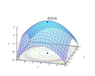
Mathematical optimization or mathematical programming is the selection of a best element, with regard to some criterion, from some set of available alternatives. It is generally divided into two subfields: discrete optimization and continuous optimization. Optimization problems arise in all quantitative disciplines from computer science and engineering to operations research and economics, and the development of solution methods has been of interest in mathematics for centuries.

Reinforcement learning (RL) is an interdisciplinary area of machine learning and optimal control concerned with how an intelligent agent ought to take actions in a dynamic environment in order to maximize the cumulative reward. Reinforcement learning is one of three basic machine learning paradigms, alongside supervised learning and unsupervised learning.

<span class="mw-page-title-main">Dynamic programming</span> Problem optimization method

Dynamic programming is both a mathematical optimization method and an algorithmic paradigm. The method was developed by Richard Bellman in the 1950s and has found applications in numerous fields, from aerospace engineering to economics.

Constraint programming (CP) is a paradigm for solving combinatorial problems that draws on a wide range of techniques from artificial intelligence, computer science, and operations research. In constraint programming, users declaratively state the constraints on the feasible solutions for a set of decision variables. Constraints differ from the common primitives of imperative programming languages in that they do not specify a step or sequence of steps to execute, but rather the properties of a solution to be found. In addition to constraints, users also need to specify a method to solve these constraints. This typically draws upon standard methods like chronological backtracking and constraint propagation, but may use customized code like a problem-specific branching heuristic.

<span class="mw-page-title-main">Optimal control</span> Mathematical way of attaining a desired output from a dynamic system

Optimal control theory is a branch of control theory that deals with finding a control for a dynamical system over a period of time such that an objective function is optimized. It has numerous applications in science, engineering and operations research. For example, the dynamical system might be a spacecraft with controls corresponding to rocket thrusters, and the objective might be to reach the Moon with minimum fuel expenditure. Or the dynamical system could be a nation's economy, with the objective to minimize unemployment; the controls in this case could be fiscal and monetary policy. A dynamical system may also be introduced to embed operations research problems within the framework of optimal control theory.

In the field of mathematical optimization, stochastic programming is a framework for modeling optimization problems that involve uncertainty. A stochastic program is an optimization problem in which some or all problem parameters are uncertain, but follow known probability distributions. This framework contrasts with deterministic optimization, in which all problem parameters are assumed to be known exactly. The goal of stochastic programming is to find a decision which both optimizes some criteria chosen by the decision maker, and appropriately accounts for the uncertainty of the problem parameters. Because many real-world decisions involve uncertainty, stochastic programming has found applications in a broad range of areas ranging from finance to transportation to energy optimization.

The Hamilton-Jacobi-Bellman (HJB) equation is a nonlinear partial differential equation that provides necessary and sufficient conditions for optimality of a control with respect to a loss function. Its solution is the value function of the optimal control problem which, once known, can be used to obtain the optimal control by taking the maximizer of the Hamiltonian involved in the HJB equation.

Pontryagin's maximum principle is used in optimal control theory to find the best possible control for taking a dynamical system from one state to another, especially in the presence of constraints for the state or input controls. It states that it is necessary for any optimal control along with the optimal state trajectory to solve the so-called Hamiltonian system, which is a two-point boundary value problem, plus a maximum condition of the control Hamiltonian. These necessary conditions become sufficient under certain convexity conditions on the objective and constraint functions.

In mathematics, a Markov decision process (MDP) is a discrete-time stochastic control process. It provides a mathematical framework for modeling decision making in situations where outcomes are partly random and partly under the control of a decision maker. MDPs are useful for studying optimization problems solved via dynamic programming. MDPs were known at least as early as the 1950s; a core body of research on Markov decision processes resulted from Ronald Howard's 1960 book, Dynamic Programming and Markov Processes. They are used in many disciplines, including robotics, automatic control, economics and manufacturing. The name of MDPs comes from the Russian mathematician Andrey Markov as they are an extension of Markov chains.
<span class="mw-page-title-main">Gauss–Newton algorithm</span> Mathematical algorithm

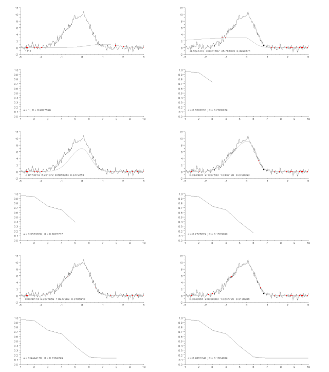
The Gauss–Newton algorithm is used to solve non-linear least squares problems, which is equivalent to minimizing a sum of squared function values. It is an extension of Newton's method for finding a minimum of a non-linear function. Since a sum of squares must be nonnegative, the algorithm can be viewed as using Newton's method to iteratively approximate zeroes of the components of the sum, and thus minimizing the sum. In this sense, the algorithm is also an effective method for solving overdetermined systems of equations. It has the advantage that second derivatives, which can be challenging to compute, are not required.

The Hamiltonian is a function used to solve a problem of optimal control for a dynamical system. It can be understood as an instantaneous increment of the Lagrangian expression of the problem that is to be optimized over a certain time period. Inspired by—but distinct from—the Hamiltonian of classical mechanics, the Hamiltonian of optimal control theory was developed by Lev Pontryagin as part of his maximum principle. Pontryagin proved that a necessary condition for solving the optimal control problem is that the control should be chosen so as to optimize the Hamiltonian.

Limited-memory BFGS is an optimization algorithm in the family of quasi-Newton methods that approximates the Broyden–Fletcher–Goldfarb–Shanno algorithm (BFGS) using a limited amount of computer memory. It is a popular algorithm for parameter estimation in machine learning. The algorithm's target problem is to minimize over unconstrained values of the real-vector where is a differentiable scalar function.

In mathematics, the theory of optimal stopping or early stopping is concerned with the problem of choosing a time to take a particular action, in order to maximise an expected reward or minimise an expected cost. Optimal stopping problems can be found in areas of statistics, economics, and mathematical finance. A key example of an optimal stopping problem is the secretary problem. Optimal stopping problems can often be written in the form of a Bellman equation, and are therefore often solved using dynamic programming.

In numerical optimization, the nonlinear conjugate gradient method generalizes the conjugate gradient method to nonlinear optimization. For a quadratic function

The value function of an optimization problem gives the value attained by the objective function at a solution, while only depending on the parameters of the problem. In a controlled dynamical system, the value function represents the optimal payoff of the system over the interval [t, t1] when started at the time-t state variable x(t)=x. If the objective function represents some cost that is to be minimized, the value function can be interpreted as the cost to finish the optimal program, and is thus referred to as "cost-to-go function." In an economic context, where the objective function usually represents utility, the value function is conceptually equivalent to the indirect utility function.

Non-linear least squares is the form of least squares analysis used to fit a set of m observations with a model that is non-linear in n unknown parameters (m ≥ n). It is used in some forms of nonlinear regression. The basis of the method is to approximate the model by a linear one and to refine the parameters by successive iterations. There are many similarities to linear least squares, but also some significant differences. In economic theory, the non-linear least squares method is applied in (i) the probit regression, (ii) threshold regression, (iii) smooth regression, (iv) logistic link regression, (v) Box–Cox transformed regressors ().

Stochastic control or stochastic optimal control is a sub field of control theory that deals with the existence of uncertainty either in observations or in the noise that drives the evolution of the system. The system designer assumes, in a Bayesian probability-driven fashion, that random noise with known probability distribution affects the evolution and observation of the state variables. Stochastic control aims to design the time path of the controlled variables that performs the desired control task with minimum cost, somehow defined, despite the presence of this noise. The context may be either discrete time or continuous time.

In machine learning, automatic basis function construction is the mathematical method of looking for a set of task-independent basis functions that map the state space to a lower-dimensional embedding, while still representing the value function accurately. Automatic basis construction is independent of prior knowledge of the domain, which allows it to perform well where expert-constructed basis functions are difficult or impossible to create.

Mean-field game theory is the study of strategic decision making by small interacting agents in very large populations. It lies at the intersection of game theory with stochastic analysis and control theory. The use of the term "mean field" is inspired by mean-field theory in physics, which considers the behavior of systems of large numbers of particles where individual particles have negligible impacts upon the system. In other words, each agent acts according to his minimization or maximization problem taking into account other agents’ decisions and because their population is large we can assume the number of agents goes to infinity and a representative agent exists.

Dynamic discrete choice (DDC) models, also known as discrete choice models of dynamic programming, model an agent's choices over discrete options that have future implications. Rather than assuming observed choices are the result of static utility maximization, observed choices in DDC models are assumed to result from an agent's maximization of the present value of utility, generalizing the utility theory upon which discrete choice models are based.

References

  1. Dixit, Avinash K. (1990). Optimization in Economic Theory (2nd ed.). Oxford University Press. p. 164. ISBN   0-19-877211-4.
  2. "Bellman's principle of optimality". www.ques10.com. Retrieved 2023-08-17.
  3. Kirk, Donald E. (1970). Optimal Control Theory: An Introduction. Prentice-Hall. p. 55. ISBN   0-13-638098-0.
  4. Szcześniak, Ireneusz; Woźna-Szcześniak, Bożena (2023), "Generic Dijkstra: Correctness and tractability", NOMS 2023-2023 IEEE/IFIP Network Operations and Management Symposium, pp. 1–7, arXiv: 2204.13547 , doi:10.1109/NOMS56928.2023.10154322, ISBN   978-1-6654-7716-1, S2CID   248427020
  5. Kirk 1970 , p.  70
  6. Kamien, Morton I.; Schwartz, Nancy L. (1991). Dynamic Optimization: The Calculus of Variations and Optimal Control in Economics and Management (Second ed.). Amsterdam: Elsevier. p. 261. ISBN   0-444-01609-0.
  7. Kirk 1970 , p.  88
  8. Jones, Morgan; Peet, Matthew M. (2020). "Extensions of the Dynamic Programming Framework: Battery Scheduling, Demand Charges, and Renewable Integration". IEEE Transactions on Automatic Control. 66 (4): 1602–1617. arXiv: 1812.00792 . doi:10.1109/TAC.2020.3002235. S2CID   119622206.
  9. Jones, Morgan; Peet, Matthew M. (2021). "A Generalization of Bellman's Equation with Application to Path Planning, Obstacle Avoidance and Invariant Set Estimation". Automatica. 127: 109510. arXiv: 2006.08175 . doi:10.1016/j.automatica.2021.109510. S2CID   222350370.
  10. 1 2 3 Bellman, R.E. (2003) [1957]. Dynamic Programming. Dover. ISBN   0-486-42809-5.
  11. 1 2 Dreyfus, S. (2002). "Richard Bellman on the birth of dynamic programming". Operations Research. 50 (1): 48–51. doi:10.1287/opre.50.1.48.17791.
  12. Bellman, 1957, Ch. III.2.
  13. Bellman, R (August 1952). "On the Theory of Dynamic Programming". Proc Natl Acad Sci U S A. 38 (8): 716–9. Bibcode:1952PNAS...38..716B. doi: 10.1073/pnas.38.8.716 . PMC   1063639 . PMID   16589166.
  14. Ljungqvist, Lars; Sargent, Thomas J. (2004). Recursive Macroeconomic Theory (2nd ed.). MIT Press. pp.  88–90. ISBN   0-262-12274-X.
  15. Bertsekas, Dimitri P.; Tsitsiklis, John N. (1996). Neuro-dynamic Programming. Athena Scientific. ISBN   978-1-886529-10-6.
  16. Abu-Khalaf, Murad; Lewis, Frank L. (2005). "Nearly optimal control laws for nonlinear systems with saturating actuators using a neural network HJB approach". Automatica. 41 (5): 779–791. doi:10.1016/j.automatica.2004.11.034. S2CID   14757582.
  17. Al-Tamimi, Asma; Lewis, Frank L.; Abu-Khalaf, Murad (2008). "Discrete-Time Nonlinear HJB Solution Using Approximate Dynamic Programming: Convergence Proof". IEEE Transactions on Systems, Man, and Cybernetics - Part B: Cybernetics. 38 (4): 943–949. doi:10.1109/TSMCB.2008.926614. PMID   18632382. S2CID   14202785.
  18. Miao, Jianjun (2014). Economic Dynamics in Discrete Time. MIT Press. p. 134. ISBN   978-0-262-32560-8.
  19. Beckmann, Martin; Muth, Richard (1954). "On the Solution to the 'Fundamental Equation' of inventory theory" (PDF). Cowles Commission Discussion Paper 2116.
  20. Merton, Robert C. (1973). "An Intertemporal Capital Asset Pricing Model". Econometrica . 41 (5): 867–887. doi:10.2307/1913811. JSTOR   1913811.
  21. Stokey, Nancy; Lucas, Robert E.; Prescott, Edward (1989). Recursive Methods in Economic Dynamics. Harvard University Press. ISBN   0-674-75096-9.
  22. Ljungqvist, Lars; Sargent, Thomas (2012). Recursive Macroeconomic Theory (3rd ed.). MIT Press. ISBN   978-0-262-01874-6.
  23. Dixit, Avinash; Pindyck, Robert (1994). Investment Under Uncertainty . Princeton University Press. ISBN   0-691-03410-9.
  24. Anderson, Patrick L. (2004). "Ch. 10". Business Economics & Finance. CRC Press. ISBN   1-58488-348-0.
    (2009). "The Value of Private Businesses in the United States". Business Economics. 44 (2): 87–108. doi:10.1057/be.2009.4. S2CID   154743445.
    (2013). Economics of Business Valuation. Stanford University Press. ISBN   9780804758307. Stanford Press Archived 2013-08-08 at the Wayback Machine
  25. Miranda, Mario J.; Fackler, Paul L. (2004). Applied Computational Economics and Finance . MIT Press. ISBN   978-0-262-29175-0.
  26. Meyn, Sean (2008). Control Techniques for Complex Networks. Cambridge University Press. ISBN   978-0-521-88441-9. Appendix contains abridged Meyn & Tweedie Archived 2007-10-12 at the Wayback Machine .