In mathematics, the Bianchi classification provides a list of all real 3-dimensional Lie algebras (up toisomorphism). The classification contains 11 classes, 9 of which contain a single Lie algebra and two of which contain a continuum-sized family of Lie algebras. (Sometimes two of the groups are included in the infinite families, giving 9 instead of 11 classes.) The classification is important in geometry and physics, because the associated Lie groups serve as symmetry groups of 3-dimensional Riemannian manifolds. It is named for Luigi Bianchi, who worked it out in 1898.
All the 3-dimensional Lie algebras other than types VIII and IX can be constructed as a semidirect product of R2 and R, with R acting on R2 by some 2 by 2 matrix M. The different types correspond to different types of matrices M, as described below.
Type I: This is the abelian and unimodular Lie algebra R3. The simply connected group has center R3 and outer automorphism group GL3(R). This is the case when M is 0.
Type II: The Heisenberg algebra, which is nilpotent and unimodular. The simply connected group has center R and outer automorphism group GL2(R). This is the case when M is nilpotent but not 0 (eigenvalues all 0).
Type III: This algebra is a product of R and the 2-dimensional non-abelian Lie algebra. (It is a limiting case of type VI, where one eigenvalue becomes zero.) It is solvable and not unimodular. The simply connected group has center R and outer automorphism group the group of non-zero real numbers. The matrix M has one zero and one non-zero eigenvalue.
Type IV: The algebra generated by [y,z] = 0, [x,y] = y, [x, z] = y + z. It is solvable and not unimodular. The simply connected group has trivial center and outer automorphism group the product of the reals and a group of order 2. The matrix M has two equal non-zero eigenvalues, but is not diagonalizable.
Type V: [y,z] = 0, [x,y] = y, [x, z] = z. Solvable and not unimodular. (A limiting case of type VI where both eigenvalues are equal.) The simply connected group has trivial center and outer automorphism group the elements of GL2(R) of determinant +1 or −1. The matrix M has two equal eigenvalues, and is diagonalizable.
Type VI: An infinite family: semidirect products of R2 by R, where the matrix M has non-zero distinct real eigenvalues with non-zero sum. The algebras are solvable and not unimodular. The simply connected group has trivial center and outer automorphism group a product of the non-zero real numbers and a group of order 2.
Type VI0: This Lie algebra is the semidirect product of R2 by R, with R where the matrix M has non-zero distinct real eigenvalues with zero sum. It is solvable and unimodular. It is the Lie algebra of the 2-dimensional Poincaré group, the group of isometries of 2-dimensional Minkowski space. The simply connected group has trivial center and outer automorphism group the product of the positive real numbers with the dihedral group of order 8.
Type VII: An infinite family: semidirect products of R2 by R, where the matrix M has non-real and non-imaginary eigenvalues. Solvable and not unimodular. The simply connected group has trivial center and outer automorphism group the non-zero reals.
Type VII0: Semidirect product of R2 by R, where the matrix M has non-zero imaginary eigenvalues. Solvable and unimodular. This is the Lie algebra of the group of isometries of the plane. The simply connected group has center Z and outer automorphism group a product of the non-zero real numbers and a group of order 2.
Type VIII: The Lie algebra sl2(R) of traceless 2 by 2 matrices, associated to the group SL2(R). It is simple and unimodular. The simply connected group is not a matrix group; it is denoted by , has center Z and its outer automorphism group has order 2.
Type IX: The Lie algebra of the orthogonal groupO3(R). It is denoted by 𝖘𝖔(3) and is simple and unimodular. The corresponding simply connected group is SU(2); it has center of order 2 and trivial outer automorphism group, and is a spin group.
The classification of 3-dimensional complex Lie algebras is similar except that types VIII and IX become isomorphic, and types VI and VII both become part of a single family of Lie algebras.
The connected 3-dimensional Lie groups can be classified as follows: they are a quotient of the corresponding simply connected Lie group by a discrete subgroup of the center, so can be read off from the table above.
The groups are related to the 8 geometries of Thurston's geometrization conjecture. More precisely, seven of the 8 geometries can be realized as a left-invariant metric on the simply connected group (sometimes in more than one way). The Thurston geometry of type S2×R cannot be realized in this way.
Structure constants
The three-dimensional Bianchi spaces each admit a set of three Killing vector fields which obey the following property:
where , the "structure constants" of the group, form a constantorder-three tensorantisymmetric in its lower two indices. For any three-dimensional Bianchi space, is given by the relationship
Figure 1. The parameter space as a 3-plane (class A) and an orthogonal half 3-plane (class B) in R with coordinates (n , n , n , a), showing the canonical representatives of each Bianchi type.
The standard Bianchi classification can be derived from the structural constants in the following six steps:
Due to the antisymmetry , there are nine independent constants . These can be equivalently represented by the nine components of an arbitrary constant matrix Cab: where εabd is the totally antisymmetric three-dimensional Levi-Civita symbol (ε123 = 1). Substitution of this expression for into the Jacobi identity, results in
The structure constants can be transformed as: Appearance of det A in this formula is due to the fact that the symbol εabd transforms as tensor density: , where έmnd ≡ εmnd. By this transformation it is always possible to reduce the matrix Cab to the form: After such a choice, one still have the freedom of making triad transformations but with the restrictions and
Now, the Jacobi identities give only one constraint:
If n1 ≠ 0 then C23 – C32 = 0 and by the remaining transformations with , the 2 × 2 matrix in Cab can be made diagonal. Then The diagonality condition for Cab is preserved under the transformations with diagonal . Under these transformations, the three parameters n1, n2, n3 change in the following way: By these diagonal transformations, the modulus of any na (if it is not zero) can be made equal to unity. Taking into account that the simultaneous change of sign of all na produce nothing new, one arrives to the following invariantly different sets for the numbers n1, n2, n3 (invariantly different in the sense that there is no way to pass from one to another by some transformation of the triad ), that is to the following different types of homogeneous spaces with diagonal matrix Cab:
Consider now the case n1 = 0. It can also happen in that case that C23 – C32 = 0. This returns to the situation already analyzed in the previous step but with the additional condition n1 = 0. Now, all essentially different types for the sets n1, n2, n3 are (0, 1, 1), (0, 1, −1), (0, 0, 1) and (0, 0, 0). The first three repeat the types VII0, VI0, II. Consequently, only one new type arises:
The only case left is n1 = 0 and C23 – C32 ≠ 0. Now the 2 × 2 matrix is non-symmetric and it cannot be made diagonal by transformations using . However, its symmetric part can be diagonalized, that is the 3 × 3 matrix Cab can be reduced to the form: where a is an arbitrary number. After this is done, there still remains the possibility to perform transformations with diagonal , under which the quantities n2, n3 and a change as follows: These formulas show that for nonzero n2, n3, a, the combination a2(n2n3)−1 is an invariant quantity. By a choice of , one can impose the condition a > 0 and after this is done, the choice of the sign of permits one to change both signs of n2 and n3 simultaneously, that is the set (n2 , n3) is equivalent to the set (−n2,−n3). It follows that there are the following four different possibilities: For the first two, the number a can be transformed to unity by a choice of the parameters and . For the second two possibilities, both of these parameters are already fixed and a remains an invariant and arbitrary positive number. Historically these four types of homogeneous spaces have been classified as: Type III is just a particular case of type VI corresponding to a = 1. Types VII and VI contain an infinity of invariantly different types of algebras corresponding to the arbitrariness of the continuous parameter a. Type VII0 is a particular case of VII corresponding to a = 0 while type VI0 is a particular case of VI corresponding also to a = 0.
Curvature of Bianchi spaces
The Bianchi spaces have the property that their Ricci tensors can be separated into a product of the basis vectors associated with the space and a coordinate-independent tensor.
(where are 1-forms), the Ricci curvature tensor is given by:
where the indices on the structure constants are raised and lowered with which is not a function of .
Cosmological application
In cosmology, this classification is used for a homogeneousspacetime of dimension 3+1. The 3-dimensional Lie group is as the symmetry group of the 3-dimensional spacelike slice, and the Lorentz metric satisfying the Einstein equation is generated by varying the metric components as a function of t. The Friedmann–Lemaître–Robertson–Walker metrics are isotropic, which are particular cases of types I, V, and IX. The Bianchi type I models include the Kasner metric as a special case. The Bianchi IX cosmologies include the Taub metric.[2] However, the dynamics near the singularity is approximately governed by a series of successive Kasner (Bianchi I) periods. The complicated dynamics, which essentially amounts to billiard motion in a portion of hyperbolic space, exhibits chaotic behaviour, and is named Mixmaster; its analysis is referred to as the BKL analysis after Belinskii, Khalatnikov and Lifshitz.[3][4] More recent work has established a relation of (super-)gravity theories near a spacelike singularity (BKL-limit) with Lorentzian Kac–Moody algebras, Weyl groups and hyperbolic Coxeter groups.[5][6][7] Other more recent work is concerned with the discrete nature of the Kasner map and a continuous generalisation.[8][9][10] In a space that is both homogeneous and isotropic the metric is determined completely, leaving free only the sign of the curvature. Assuming only space homogeneity with no additional symmetry such as isotropy leaves considerably more freedom in choosing the metric. The following pertains to the space part of the metric at a given instant of time t assuming a synchronous frame so that t is the same synchronised time for the whole space.
Homogeneity implies identical metric properties at all points of the space. An exact definition of this concept involves considering sets of coordinate transformations that transform the space into itself, i.e. leave its metric unchanged: if the line element before transformation is
then after transformation the same line element is
with the same functional dependence of γαβ on the new coordinates. (For a more theoretical and coordinate-independent definition of homogeneous space see homogeneous space). A space is homogeneous if it admits a set of transformations (a group of motions) that brings any given point to the position of any other point. Since space is three-dimensional the different transformations of the group are labelled by three independent parameters.
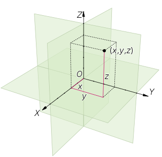
Figure 2. The triad e (e , e , e ) is an affine coordinate system (including as a special case Cartesian coordinate system) whose coordinates are functions of the curvilinear coordinates xα (x1, x2, x3).
In Euclidean space the homogeneity of space is expressed by the invariance of the metric under parallel displacements (translations) of the Cartesian coordinate system. Each translation is determined by three parameters — the components of the displacement vector of the coordinate origin. All these transformations leave invariant the three independent differentials (dx, dy, dz) from which the line element is constructed. In the general case of a non-Euclidean homogeneous space, the transformations of its group of motions again leave invariant three independent linear differential forms, which do not, however, reduce to total differentials of any coordinate functions. These forms are written as where the Latin index (a) labels three independent vectors (coordinate functions); these vectors are called a frame field or triad. The Greek letters label the three space-like curvilinear coordinates. A spatial metric invariant is constructed under the given group of motions with the use of the above forms:
(eq. 6a)
i.e. the metric tensor is
(eq. 6b)
where the coefficients ηab, which are symmetric in the indices a and b, are functions of time. The choice of basis vectors is dictated by the symmetry properties of the space and, in general, these basis vectors are not orthogonal (so that the matrix ηab is not diagonal).
The reciprocal triple of vectors is introduced with the help of Kronecker delta
(eq. 6c)
In the three-dimensional case, the relation between the two vector triples can be written explicitly
(eq. 6d)
where the volume v is
with e(a) and e(a) regarded as Cartesian vectors with components and , respectively. The determinant of the metric tensor eq. 6b is γ = ηv2 where η is the determinant of the matrix ηab.
The required conditions for the homogeneity of the space are
The invariance of the differential forms means that
where the on the two sides of the equation are the same functions of the old and new coordinates, respectively. Multiplying this equation by , setting and comparing coefficients of the same differentials dxα, one finds
These equations are a system of differential equations that determine the functions for a given frame. In order to be integrable, these equations must satisfy identically the conditions
Calculating the derivatives, one finds
Multiplying both sides of the equations by and shifting the differentiation from one factor to the other by using eq. 6c, one gets for the left side:
and for the right, the same expression in the variable x. Since x and x' are arbitrary, these expression must reduce to constants to obtain eq. 6e.
Multiplying by , eq. 6e can be rewritten in the form
where again the vector operations are done as if the coordinates xα were Cartesian. Using eq. 6d, one obtains
(eq. 6g)
and six more equations obtained by a cyclic permutation of indices 1, 2, 3.
The structure constants are antisymmetric in their lower indices as seen from their definition eq. 6e: . Another condition on the structure constants can be obtained by noting that eq. 6f can be written in the form of commutation relations
In the mathematical theory of continuous groups (Lie groups) the operators Xa satisfying conditions eq. 6h are called the generators of the group. The theory of Lie groups uses operators defined using the Killing vectors instead of triads . Since in the synchronous metric none of the γαβ components depends on time, the Killing vectors (triads) are time-like.
It is a definite advantage to use, in place of the three-index constants , a set of two-index quantities, obtained by the dual transformation
(eq. 6k)
where eabc = eabc is the unit antisymmetric symbol (with e123 = +1). With these constants the commutation relations eq. 6h are written as
(eq. 6l)
The antisymmetry property is already taken into account in the definition eq. 6k, while property eq. 6j takes the form
(eq. 6m)
The choice of the three frame vectors in the differential forms (and with them the operators Xa) is not unique. They can be subjected to any linear transformation with constant coefficients:
(eq. 6n)
The quantities ηab and Cab behave like tensors (are invariant) with respect to such transformations.
The conditions eq. 6m are the only ones that the structure constants must satisfy. But among the constants admissible by these conditions, there are equivalent sets, in the sense that their difference is related to a transformation of the type eq. 6n. The question of the classification of homogeneous spaces reduces to determining all nonequivalent sets of structure constants. This can be done, using the "tensor" properties of the quantities Cab, by the following simple method (C. G. Behr, 1962).
The asymmetric tensor Cab can be resolved into a symmetric and an antisymmetric part. The first is denoted by nab, and the second is expressed in terms of its dual vectorac:
(eq. 6o)
Substitution of this expression in eq. 6m leads to the condition
(eq. 6p)
By means of the transformations eq. 6n the symmetric tensor nab can be brought to diagonal form with eigenvaluesn1, n2, n3. Equation 6p shows that the vector ab (if it exists) lies along one of the principal directions of the tensor nab, the one corresponding to the eigenvalue zero. Without loss of generality one can therefore set ab = (a, 0, 0). Then eq. 6p reduces to an1 = 0, i.e. one of the quantities a or n1 must be zero. The Jacobi identities take the form:
(eq. 6q)
The only remaining freedoms are sign changes of the operators Xa and their multiplication by arbitrary constants. This permits to simultaneously change the sign of all the na and also to make the quantity a positive (if it is different from zero). Also all structure constants can be made equal to ±1, if at least one of the quantities a, n2, n3 vanishes. But if all three of these quantities differ from zero, the scale transformations leave invariant the ratio h = a2(n2n3)−1.
Thus one arrives at the Bianchi classification listing the possible types of homogeneous spaces classified by the values of a, n1, n2, n3 which is graphically presented in Fig. 3. In the class A case (a = 0), type IX (n(1)=1, n(2)=1, n(3)=1) is represented by octant 2, type VIII (n(1)=1, n(2)=1, n(3)=–1) is represented by octant 6, while type VII0 (n(1)=1, n(2)=1, n(3)=0) is represented by the first quadrant of the horizontal plane and type VI0 (n(1)=1, n(2)=–1, n(3)=0) is represented by the fourth quadrant of this plane; type II ((n(1)=1, n(2)=0, n(3)=0) is represented by the interval [0,1] along n(1) and type I (n(1)=0, n(2)=0, n(3)=0) is at the origin. Similarly in the class B case (with n(3) = 0), Bianchi type VIh (a=h, n(1)=1, n(2)=–1) projects to the fourth quadrant of the horizontal plane and type VIIh (a=h, n(1)=1, n(2)=1) projects to the first quadrant of the horizontal plane; these last two types are a single isomorphism class corresponding to a constant value surface of the function h = a2(n(1)n(2))−1. A typical such surface is illustrated in one octant, the angle θ given by tanθ = |h/2|1/2; those in the remaining octants are obtained by rotation through multiples of π/2, h alternating in sign for a given magnitude |h|. Type III is a subtype of VIh with a=1. Type V (a=1, n(1)=0, n(2)=0) is the interval (0,1] along the axis a and type IV (a=1, n(1)=1, n(2)=0) is the vertical open face between the first and fourth quadrants of the a = 0 plane with the latter giving the class A limit of each type.
The Einstein equations for a universe with a homogeneous space can reduce to a system of ordinary differential equations containing only functions of time with the help of a frame field. To do this one must resolve the spatial components of four-vectors and four-tensors along the triad of basis vectors of the space:
where all these quantities are now functions of t alone; the scalar quantities, the energy density ε and the pressure of the matter p, are also functions of the time.
The Einstein equations in vacuum in synchronous reference frame are[11][12][note 1]
(eq. 11)
(eq. 12)
(eq. 13)
where is the 3-dimensional tensor , and Pαβ is the 3-dimensional Ricci tensor, which is expressed by the 3-dimensional metric tensor γαβ in the same way as Rik is expressed by gik; Pαβ contains only the space (but not the time) derivatives of γαβ. Using triads, for eq. 11 one has simply
The components of P(a)(b) can be expressed in terms of the quantities ηab and the structure constants of the group by using the tetrad representation of the Ricci tensor in terms of quantities [13]
After replacing the three-index symbols by two-index symbols Cab and the transformations:
one gets the "homogeneous" Ricci tensor expressed in structure constants:
Here, all indices are raised and lowered with the local metric tensor ηab
The Bianchi identities for the three-dimensional tensor Pαβ in the homogeneous space take the form
Taking into account the transformations of covariant derivatives for arbitrary four-vectors Ai and four-tensors Aik
the final expressions for the triad components of the Ricci four-tensor are:
(eq. 11a)
(eq. 12a)
(eq. 13a)
In setting up the Einstein equations there is thus no need to use explicit expressions for the basis vectors as functions of the coordinates.
↑ The convention used by BKL is the same as in the Landau & Lifshitz (1988) book. The Latin indices run through the values 0, 1, 2, 3; Greek indices run through the space values 1, 2, 3. The metric gik has the signature (+ − − −); γαβ = −gαβ is the 3-dimensional space metric tensor. BKL use a system of units, in which the speed of light and the Einstein gravitational constant are equal to 1.
Related Research Articles
Euclidean space is the fundamental space of geometry, intended to represent physical space. Originally, that is, in Euclid's Elements, it was the three-dimensional space of Euclidean geometry, but in modern mathematics there are Euclidean spaces of any positive integer dimension, including the three-dimensional space and the Euclidean plane. The qualifier "Euclidean" is used to distinguish Euclidean spaces from other spaces that were later considered in physics and modern mathematics.
In mathematics, an operator is generally a mapping or function that acts on elements of a space to produce elements of another space. There is no general definition of an operator, but the term is often used in place of function when the domain is a set of functions or other structured objects. Also, the domain of an operator is often difficult to be explicitly characterized, and may be extended to related objects. See Operator (physics) for other examples.
In mathematics, a tensor is an algebraic object that describes a multilinear relationship between sets of algebraic objects related to a vector space. Tensors may map between different objects such as vectors, scalars, and even other tensors. There are many types of tensors, including scalars and vectors, dual vectors, multilinear maps between vector spaces, and even some operations such as the dot product. Tensors are defined independent of any basis, although they are often referred to by their components in a basis related to a particular coordinate system.
In the mathematical field of differential geometry, the Riemann curvature tensor or Riemann–Christoffel tensor is the most common way used to express the curvature of Riemannian manifolds. It assigns a tensor to each point of a Riemannian manifold. It is a local invariant of Riemannian metrics which measures the failure of the second covariant derivatives to commute. A Riemannian manifold has zero curvature if and only if it is flat, i.e. locally isometric to the Euclidean space. The curvature tensor can also be defined for any pseudo-Riemannian manifold, or indeed any manifold equipped with an affine connection.
In multilinear algebra, a tensor contraction is an operation on a tensor that arises from the natural pairing of a finite-dimensional vector space and its dual. In components, it is expressed as a sum of products of scalar components of the tensor(s) caused by applying the summation convention to a pair of dummy indices that are bound to each other in an expression. The contraction of a single mixed tensor occurs when a pair of literal indices of the tensor are set equal to each other and summed over. In Einstein notation this summation is built into the notation. The result is another tensor with order reduced by 2.
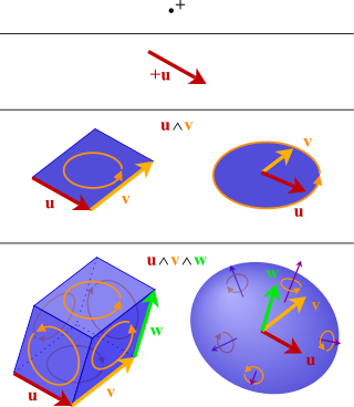
In mathematics, the exterior algebra, or Grassmann algebra, named after Hermann Grassmann, is an algebra that uses the exterior product or wedge product as its multiplication. In mathematics, the exterior product or wedge product of vectors is an algebraic construction used in geometry to study areas, volumes, and their higher-dimensional analogues. The exterior product of two vectors and denoted by is called a bivector and lives in a space called the exterior square, a vector space that is distinct from the original space of vectors. The magnitude of can be interpreted as the area of the parallelogram with sides and which in three dimensions can also be computed using the cross product of the two vectors. More generally, all parallel plane surfaces with the same orientation and area have the same bivector as a measure of their oriented area. Like the cross product, the exterior product is anticommutative, meaning that for all vectors and but, unlike the cross product, the exterior product is associative.
In mathematical physics, Minkowski space combines inertial space and time manifolds (x,y) with a non-inertial reference frame of space and time (x',t') into a four-dimensional model relating a position to the field (physics). A four-vector (x,y,z,t) consisting of coordinate axes such as a Euclidean space plus time may be used with the non-inertial frame to illustrate specifics of motion, but should not be confused with the spacetime model generally. The model helps show how a spacetime interval between any two events is independent of the inertial frame of reference in which they are recorded. Although initially developed by mathematician Hermann Minkowski for Maxwell's equations of electromagnetism, the mathematical structure of Minkowski spacetime was shown to be implied by the postulates of special relativity.
In differential geometry, the Ricci curvature tensor, named after Gregorio Ricci-Curbastro, is a geometric object which is determined by a choice of Riemannian or pseudo-Riemannian metric on a manifold. It can be considered, broadly, as a measure of the degree to which the geometry of a given metric tensor differs locally from that of ordinary Euclidean space or pseudo-Euclidean space.
In differential geometry, the Lie derivative, named after Sophus Lie by Władysław Ślebodziński, evaluates the change of a tensor field, along the flow defined by another vector field. This change is coordinate invariant and therefore the Lie derivative is defined on any differentiable manifold.
In mathematics, particularly in the theories of Lie groups, algebraic groups and topological groups, a homogeneous space for a group G is a non-empty manifold or topological space X on which G acts transitively. The elements of G are called the symmetries of X. A special case of this is when the group G in question is the automorphism group of the space X – here "automorphism group" can mean isometry group, diffeomorphism group, or homeomorphism group. In this case, X is homogeneous if intuitively X looks locally the same at each point, either in the sense of isometry, diffeomorphism, or homeomorphism (topology). Some authors insist that the action of G be faithful, although the present article does not. Thus there is a group action of G on X which can be thought of as preserving some "geometric structure" on X, and making X into a single G-orbit.
In mathematics, the covariant derivative is a way of specifying a derivative along tangent vectors of a manifold. Alternatively, the covariant derivative is a way of introducing and working with a connection on a manifold by means of a differential operator, to be contrasted with the approach given by a principal connection on the frame bundle – see affine connection. In the special case of a manifold isometrically embedded into a higher-dimensional Euclidean space, the covariant derivative can be viewed as the orthogonal projection of the Euclidean directional derivative onto the manifold's tangent space. In this case the Euclidean derivative is broken into two parts, the extrinsic normal component and the intrinsic covariant derivative component.
In mathematics, a Killing vector field, named after Wilhelm Killing, is a vector field on a Riemannian manifold that preserves the metric. Killing fields are the infinitesimal generators of isometries; that is, flows generated by Killing fields are continuous isometries of the manifold. More simply, the flow generates a symmetry, in the sense that moving each point of an object the same distance in the direction of the Killing vector will not distort distances on the object.
When studying and formulating Albert Einstein's theory of general relativity, various mathematical structures and techniques are utilized. The main tools used in this geometrical theory of gravitation are tensor fields defined on a Lorentzian manifold representing spacetime. This article is a general description of the mathematics of general relativity.
In differential geometry and theoretical physics, the Petrov classification describes the possible algebraic symmetries of the Weyl tensor at each event in a Lorentzian manifold.
In mathematics, a differentiable manifold is a type of manifold that is locally similar enough to a vector space to allow one to apply calculus. Any manifold can be described by a collection of charts (atlas). One may then apply ideas from calculus while working within the individual charts, since each chart lies within a vector space to which the usual rules of calculus apply. If the charts are suitably compatible, then computations done in one chart are valid in any other differentiable chart.
In differential geometry and mathematical physics, a spin connection is a connection on a spinor bundle. It is induced, in a canonical manner, from the affine connection. It can also be regarded as the gauge field generated by local Lorentz transformations. In some canonical formulations of general relativity, a spin connection is defined on spatial slices and can also be regarded as the gauge field generated by local rotations.
A Belinski–Khalatnikov–Lifshitz (BKL) singularity is a model of the dynamic evolution of the universe near the initial gravitational singularity, described by an anisotropic, chaotic solution of the Einstein field equation of gravitation. According to this model, the universe is chaotically oscillating around a gravitational singularity in which time and space become equal to zero or, equivalently, the spacetime curvature becomes infinitely big. This singularity is physically real in the sense that it is a necessary property of the solution, and will appear also in the exact solution of those equations. The singularity is not artificially created by the assumptions and simplifications made by the other special solutions such as the Friedmann–Lemaître–Robertson–Walker, quasi-isotropic, and Kasner solutions.
The tetrad formalism is an approach to general relativity that generalizes the choice of basis for the tangent bundle from a coordinate basis to the less restrictive choice of a local basis, i.e. a locally defined set of four linearly independent vector fields called a tetrad or vierbein. It is a special case of the more general idea of a vielbein formalism, which is set in (pseudo-)Riemannian geometry. This article as currently written makes frequent mention of general relativity; however, almost everything it says is equally applicable to (pseudo-)Riemannian manifolds in general, and even to spin manifolds. Most statements hold simply by substituting arbitrary for . In German, "vier" translates to "four", and "viel" to "many".
In mathematics, the structure constants or structure coefficients of an algebra over a field are used to explicitly specify the product of two basis vectors in the algebra as a linear combination. Given the structure constants, the resulting product is bilinear and can be uniquely extended to all vectors in the vector space, thus uniquely determining the product for the algebra.
A synchronous frame is a reference frame in which the time coordinate defines proper time for all co-moving observers. It is built by choosing some constant time hypersurface as an origin, such that has in every point a normal along the time line and a light cone with an apex in that point can be constructed; all interval elements on this hypersurface are space-like. A family of geodesics normal to this hypersurface are drawn and defined as the time coordinates with a beginning at the hypersurface. In terms of metric-tensor components , a synchronous frame is defined such that
L. Bianchi, Sugli spazi a tre dimensioni che ammettono un gruppo continuo di movimenti. (On the spaces of three dimensions that admit a continuous group of movements.) Soc. Ital. Sci. Mem. di Mat. 11, 267 (1898) English translationArchived 2020-02-18 at the Wayback Machine
Guido Fubini Sugli spazi a quattro dimensioni che ammettono un gruppo continuo di movimenti, (On the spaces of four dimensions that admit a continuous group of movements.) Ann. Mat. pura appli. (3) 9, 33-90 (1904); reprinted in Opere Scelte, a cura dell'Unione matematica italiana e col contributo del Consiglio nazionale delle ricerche, Roma Edizioni Cremonese, 1957–62
MacCallum, On the classification of the real four-dimensional Lie algebras, in "On Einstein's path: essays in honor of Engelbert Schucking" edited by A. L. Harvey, Springer ISBN0-387-98564-6
This page is based on this Wikipedia article Text is available under the CC BY-SA 4.0 license; additional terms may apply. Images, videos and audio are available under their respective licenses.