Characterizations of the exponential function

In mathematics, the exponential function can be characterized in many ways. The following characterizations (definitions) are most common. This article discusses why each characterization makes sense, and why they are all equivalent to each other. As a special case of these considerations, it will be demonstrated that the three most common definitions for the mathematical constant e are equivalent to each other.

Characterizations

The six most common definitions of the exponential function ${\displaystyle \exp(x)=e^{x}}$ for real values ${\displaystyle x\in \mathbb {R} }$ are as follows.

1. Product limit. Define ${\displaystyle e^{x}}$ by the limit:
   $${\displaystyle e^{x}=\lim _{n\to \infty }\left(1+{\frac {x}{n}}\right)^{n}.}$$
2. Power series. Define e^x as the value of the infinite series
   $${\displaystyle e^{x}=\sum _{n=0}^{\infty }{x^{n} \over n!}=1+x+{\frac {x^{2}}{2!}}+{\frac {x^{3}}{3!}}+{\frac {x^{4}}{4!}}+\cdots }$$
   (Here n! denotes the factorial of n. One proof that e is irrational uses a special case of this formula.)
3. Inverse of logarithm integral. Define ${\displaystyle e^{x}}$ to be the unique number y > 0 such that
   $${\displaystyle \int _{1}^{y}{\frac {dt}{t}}=x.}$$
   That is, ${\displaystyle e^{x}}$ is the inverse of the natural logarithm function ${\displaystyle x=\ln(y)}$, which is defined by this integral.
4. Differential equation. Define ${\displaystyle y(x)=e^{x}}$ to be the unique solution to the differential equation with initial value:
   $${\displaystyle y'=y,\quad y(0)=1,}$$
   where ${\displaystyle y'={\tfrac {dy}{dx}}}$ denotes the derivative of y.
5. Functional equation. The exponential function ${\displaystyle e^{x}}$ is the unique function f with ${\displaystyle f(x+y)=f(x)f(y)}$ for all ${\displaystyle x,y}$ and ${\displaystyle f'(0)=1}$. The condition ${\displaystyle f'(0)=1}$ can be replaced with ${\displaystyle f(1)=e}$ together with any of the following regularity conditions:
   • f is Lebesgue-measurable (Hewitt and Stromberg, 1965, exercise 18.46).
   • f is continuous at any one point (Rudin, 1976, chapter 8, exercise 6).
   • f is increasing.
   For the uniqueness, one must impose some regularity condition, since other functions satisfying ${\displaystyle f(x+y)=f(x)f(y)}$ can be constructed using a basis for the real numbers over the rationals, as described by Hewitt and Stromberg.
6. Elementary definition by powers. Define the exponential function with base ${\displaystyle a>0}$ to be the continuous function ${\displaystyle a^{x}}$ whose value on integers ${\displaystyle x=n}$ is given by repeated multipication or division of ${\displaystyle a}$, and whose value on rational numbers ${\displaystyle x=n/m}$ is given by ${\displaystyle a^{n/m}=\ \ {\sqrt[{m}]{{\vphantom {A^{2}}}a^{n}}}}$. Then define ${\displaystyle e^{x}}$ to be the exponential function whose base ${\displaystyle a=e}$ is the unique positive real number satisfying:
   $${\displaystyle \lim _{h\to 0}{\frac {e^{h}-1}{h}}=1.}$$

Larger domains

One way of defining the exponential function over the complex numbers is to first define it for the domain of real numbers using one of the above characterizations, and then extend it as an analytic function, which is characterized by its values on any infinite domain set.

Also, characterisations (1), (2), and (4) for ${\displaystyle e^{x}}$ apply directly for ${\displaystyle x}$ a complex number. Definition (3) presents a problem because there are non-equivalent paths along which one could integrate; but the equation of (3) should hold for any such path modulo ${\displaystyle 2\pi }$. As for definition (5), the additive property together with the complex derivative ${\displaystyle f'(0)=1}$ are sufficient to guarantee ${\displaystyle f(x)=e^{x}}$. However, the initial value condition ${\displaystyle f(1)=e}$ together with the other regularity conditions are not sufficient. For example, for real x and y, the function

$${\displaystyle f(x+iy)=e^{x}(\cos(2y)+i\sin(2y))=e^{x+2iy}}$$

satisfies the three listed regularity conditions in (5) but is not equal to ${\displaystyle \exp(x+iy)}$. A sufficient condition is that ${\displaystyle f(1)=e}$ and that f is a conformal map at some point; or else the two initial values ${\displaystyle f(1)=e}$ and ${\textstyle f(i)=\cos(1)+i\sin(1)}$ together with the other regularity conditions.

One may also define the exponential on other domains, such as matrices and other algebras. Definitions (1), (2), and (4) all make sense for arbitrary Banach algebras.

Proof that each characterization makes sense

Some of these definitions require justification to demonstrate that they are well-defined. For example, when the value of the function is defined as the result of a limiting process (i.e. an infinite sequence or series), it must be demonstrated that such a limit always exists.

Characterization 1

The error of the product limit expression is described by:

$${\displaystyle \left(1+{\frac {x}{n}}\right)^{n}=e^{x}\left(1-{\frac {x^{2}}{2n}}+{\frac {x^{3}(8+3x)}{24n^{2}}}+\cdots \right),}$$

where the polynomial's degree (in x) in the term with denominator n^k is 2k.

Characterization 2

Since

$${\displaystyle \lim _{n\to \infty }\left|{\frac {x^{n+1}/(n+1)!}{x^{n}/n!}}\right|=\lim _{n\to \infty }\left|{\frac {x}{n+1}}\right|=0<1.}$$

it follows from the ratio test that ${\textstyle \sum _{n=0}^{\infty }{\frac {x^{n}}{n!}}}$ converges for all x.

Characterization 3

Since the integrand is an integrable function of t, the integral expression is well-defined. It must be shown that the function from ${\displaystyle \mathbb {R} ^{+}}$ to ${\displaystyle \mathbb {R} }$ defined by

$${\displaystyle x\mapsto \int _{1}^{x}{\frac {dt}{t}}}$$

is a bijection. Since 1/t is positive for positive t, this function is strictly increasing, hence injective. If the two integrals

$${\displaystyle {\begin{aligned}\int _{1}^{\infty }{\frac {dt}{t}}&=\infty \\[8pt]\int _{1}^{0}{\frac {dt}{t}}&=-\infty \end{aligned}}}$$

hold, then it is surjective as well. Indeed, these integrals do hold; they follow from the integral test and the divergence of the harmonic series.

Characterization 6

The defnition depends on the unique positive real number ${\displaystyle a=e}$ satisfying:

$${\displaystyle \lim _{h\to 0}{\frac {a^{h}-1}{h}}=1.}$$

This limit can be shown to exist for any ${\displaystyle a}$, and it defines a continuous increasing function ${\displaystyle f(a)=\ln(a)}$ with ${\displaystyle f(1)=0}$ and ${\displaystyle \lim _{a\to \infty }f(a)=\infty }$, so the Intermediate value theorem guarantees the existence of such a value ${\displaystyle a=e}$.

Equivalence of the characterizations

The following arguments demonstrate the equivalence of the above characterizations for the exponential function.

Characterization 1 ⇔ characterization 2

The following argument is adapted from Rudin, theorem 3.31, p. 63–65.

Let ${\displaystyle x\geq 0}$ be a fixed non-negative real number. Define

$${\displaystyle t_{n}=\left(1+{\frac {x}{n}}\right)^{n},\qquad s_{n}=\sum _{k=0}^{n}{\frac {x^{k}}{k!}},\qquad e^{x}=\lim _{n\to \infty }s_{n}.}$$

By the binomial theorem,

$${\displaystyle {\begin{aligned}t_{n}&=\sum _{k=0}^{n}{n \choose k}{\frac {x^{k}}{n^{k}}}=1+x+\sum _{k=2}^{n}{\frac {n(n-1)(n-2)\cdots (n-(k-1))x^{k}}{k!\,n^{k}}}\\[8pt]&=1+x+{\frac {x^{2}}{2!}}\left(1-{\frac {1}{n}}\right)+{\frac {x^{3}}{3!}}\left(1-{\frac {1}{n}}\right)\left(1-{\frac {2}{n}}\right)+\cdots \\[8pt]&{}\qquad \cdots +{\frac {x^{n}}{n!}}\left(1-{\frac {1}{n}}\right)\cdots \left(1-{\frac {n-1}{n}}\right)\leq s_{n}\end{aligned}}}$$

(using x ≥ 0 to obtain the final inequality) so that:

$${\displaystyle \limsup _{n\to \infty }t_{n}\leq \limsup _{n\to \infty }s_{n}=e^{x}}$$

One must use lim sup because it is not known if t_n converges.

For the other inequality, by the above expression for t_n, if 2 ≤ m ≤ n, we have:

$${\displaystyle 1+x+{\frac {x^{2}}{2!}}\left(1-{\frac {1}{n}}\right)+\cdots +{\frac {x^{m}}{m!}}\left(1-{\frac {1}{n}}\right)\left(1-{\frac {2}{n}}\right)\cdots \left(1-{\frac {m-1}{n}}\right)\leq t_{n}.}$$

Fix m, and let n approach infinity. Then

$${\displaystyle s_{m}=1+x+{\frac {x^{2}}{2!}}+\cdots +{\frac {x^{m}}{m!}}\leq \liminf _{n\to \infty }\ t_{n}}$$

(again, one must use lim inf because it is not known if t_n converges). Now, take the above inequality, let m approach infinity, and put it together with the other inequality to obtain:

$${\displaystyle \limsup _{n\to \infty }t_{n}\leq e^{x}\leq \liminf _{n\to \infty }t_{n}}$$

so that

$${\displaystyle \lim _{n\to \infty }t_{n}=e^{x}.}$$

This equivalence can be extended to the negative real numbers by noting ${\textstyle \left(1-{\frac {r}{n}}\right)^{n}\left(1+{\frac {r}{n}}\right)^{n}=\left(1-{\frac {r^{2}}{n^{2}}}\right)^{n}}$ and taking the limit as n goes to infinity.

Characterization 1 ⇔ characterization 3

Here, the natural logarithm function is defined in terms of a definite integral as above. By the first part of fundamental theorem of calculus,

$${\displaystyle {\frac {d}{dx}}\ln x={\frac {d}{dx}}\int _{1}^{x}{\frac {1}{t}}\,dt={\frac {1}{x}}.}$$

Besides, ${\textstyle \ln 1=\int _{1}^{1}{\frac {dt}{t}}=0}$

Now, let x be any fixed real number, and let

$${\displaystyle y=\lim _{n\to \infty }\left(1+{\frac {x}{n}}\right)^{n}.}$$

Ln(y) = x, which implies that y = e^x, where e^x is in the sense of definition 3. We have

$${\displaystyle \ln y=\ln \lim _{n\to \infty }\left(1+{\frac {x}{n}}\right)^{n}=\lim _{n\to \infty }\ln \left(1+{\frac {x}{n}}\right)^{n}.}$$

Here, the continuity of ln(y) is used, which follows from the continuity of 1/t:

$${\displaystyle \ln y=\lim _{n\to \infty }n\ln \left(1+{\frac {x}{n}}\right)=\lim _{n\to \infty }{\frac {x\ln \left(1+(x/n)\right)}{(x/n)}}.}$$

Here, the result lnaⁿ = nlna has been used. This result can be established for n a natural number by induction, or using integration by substitution. (The extension to real powers must wait until ln and exp have been established as inverses of each other, so that a^b can be defined for real b as e^{b lna}.)

$${\displaystyle =x\cdot \lim _{h\to 0}{\frac {\ln \left(1+h\right)}{h}}\quad {\text{ where }}h={\frac {x}{n}}}$$

$${\displaystyle =x\cdot \lim _{h\to 0}{\frac {\ln \left(1+h\right)-\ln 1}{h}}}$$

$${\displaystyle =x\cdot {\frac {d}{dt}}\ln t{\Bigg |}_{t=1}}$$

$${\displaystyle \!\,=x.}$$

Characterization 1 ⇔ characterization 4

Let ${\displaystyle y(t)}$ denote the solution to the initial value problem ${\displaystyle y'=y,\ y(0)=1}$. Applying the simplest form of Euler's method with increment ${\displaystyle \Delta t={\frac {x}{n}}}$ and sample points ${\displaystyle t\ =\ 0,\ \Delta t,\ 2\Delta t,\ldots ,\ n\Delta t}$ gives the recursive formula:

${\displaystyle y(t+\Delta t)\ \approx \ y(t)+y'(t)\Delta t\ =\ y(t)+y(t)\Delta t\ =\ y(t)\,(1+\Delta t).}$

This recursion is immediately solved to give the approximate value ${\displaystyle y(x)=y(n\Delta t)\approx (1+\Delta t)^{n}}$, and since Euler's Method is known to converge to the exact solution, we have:

${\displaystyle y(x)=\lim _{n\to \infty }\left(1+{\frac {x}{n}}\right)^{n}.}$

Characterization 1 ⇔ characterization 5

The following proof is a simplified version of the one in Hewitt and Stromberg, exercise 18.46. First, one proves that measurability (or here, Lebesgue-integrability) implies continuity for a non-zero function ${\displaystyle f(x)}$ satisfying ${\displaystyle f(x+y)=f(x)f(y)}$, and then one proves that continuity implies ${\displaystyle f(x)=e^{kx}}$ for some k, and finally ${\displaystyle f(1)=e}$ implies k = 1.

First, a few elementary properties from ${\displaystyle f(x)}$ satisfying ${\displaystyle f(x+y)=f(x)f(y)}$ are proven, and the assumption that ${\displaystyle f(x)}$ is not identically zero:

• If ${\displaystyle f(x)}$ is nonzero anywhere (say at x=y), then it is non-zero everywhere. Proof: ${\displaystyle f(y)=f(x)f(y-x)\neq 0}$ implies ${\displaystyle f(x)\neq 0}$.
• ${\displaystyle f(0)=1}$. Proof: ${\displaystyle f(x)=f(x+0)=f(x)f(0)}$ and ${\displaystyle f(x)}$ is non-zero.
• ${\displaystyle f(-x)=1/f(x)}$. Proof: ${\displaystyle 1=f(0)=f(x-x)=f(x)f(-x)}$.
• If ${\displaystyle f(x)}$ is continuous anywhere (say at x = y), then it is continuous everywhere. Proof: ${\displaystyle f(x+\delta )-f(x)=f(x-y)[f(y+\delta )-f(y)]\to 0}$ as ${\displaystyle \delta \to 0}$ by continuity at y.

The second and third properties mean that it is sufficient to prove ${\displaystyle f(x)=e^{x}}$ for positive x.

If ${\displaystyle f(x)}$ is a Lebesgue-integrable function, then

$${\displaystyle g(x)=\int _{0}^{x}f(x')\,dx'.}$$

It then follows that

$${\displaystyle g(x+y)-g(x)=\int _{x}^{x+y}f(x')\,dx'=\int _{0}^{y}f(x+x')\,dx'=f(x)g(y).}$$

Since ${\displaystyle f(x)}$ is nonzero, some y can be chosen such that ${\displaystyle g(y)\neq 0}$ and solve for ${\displaystyle f(x)}$ in the above expression. Therefore:

$${\displaystyle {\begin{aligned}f(x+\delta )-f(x)&={\frac {[g(x+\delta +y)-g(x+\delta )]-[g(x+y)-g(x)]}{g(y)}}\\&={\frac {[g(x+y+\delta )-g(x+y)]-[g(x+\delta )-g(x)]}{g(y)}}\\&={\frac {f(x+y)g(\delta )-f(x)g(\delta )}{g(y)}}=g(\delta ){\frac {f(x+y)-f(x)}{g(y)}}.\end{aligned}}}$$

The final expression must go to zero as ${\displaystyle \delta \to 0}$ since ${\displaystyle g(0)=0}$ and ${\displaystyle g(x)}$ is continuous. It follows that ${\displaystyle f(x)}$ is continuous.

Now, ${\displaystyle f(q)=e^{kq}}$ can be proven, for some k, for all positive rational numbers q. Let q=n/m for positive integers n and m. Then

$${\displaystyle f\left({\frac {n}{m}}\right)=f\left({\frac {1}{m}}+\cdots +{\frac {1}{m}}\right)=f\left({\frac {1}{m}}\right)^{n}}$$

by elementary induction on n. Therefore, ${\displaystyle f(1/m)^{m}=f(1)}$ and thus

$${\displaystyle f\left({\frac {n}{m}}\right)=f(1)^{n/m}=e^{k(n/m)}.}$$

for ${\displaystyle k=\ln[f(1)]}$. If restricted to real-valued ${\displaystyle f(x)}$, then ${\displaystyle f(x)=f(x/2)^{2}}$ is everywhere positive and so k is real.

Finally, by continuity, since ${\displaystyle f(x)=e^{kx}}$ for all rational x, it must be true for all real x since the closure of the rationals is the reals (that is, any real x can be written as the limit of a sequence of rationals). If ${\displaystyle f(1)=e}$ then k = 1. This is equivalent to characterization 1 (or 2, or 3), depending on which equivalent definition of e one uses.

Characterization 2 ⇔ characterization 4

Let n be a non-negative integer. In the sense of definition 4 and by induction, ${\displaystyle {\frac {d^{n}y}{dx^{n}}}=y}$.

Therefore ${\displaystyle {\frac {d^{n}y}{dx^{n}}}{\Bigg |}_{x=0}=y(0)=1.}$

Using Taylor series,

$${\displaystyle y=\sum _{n=0}^{\infty }{\frac {f^{(n)}(0)}{n!}}\,x^{n}=\sum _{n=0}^{\infty }{\frac {1}{n!}}\,x^{n}=\sum _{n=0}^{\infty }{\frac {x^{n}}{n!}}.}$$

This shows that definition 4 implies definition 2.

In the sense of definition 2,

$${\displaystyle {\begin{aligned}{\frac {d}{dx}}e^{x}&={\frac {d}{dx}}\left(1+\sum _{n=1}^{\infty }{\frac {x^{n}}{n!}}\right)=\sum _{n=1}^{\infty }{\frac {nx^{n-1}}{n!}}=\sum _{n=1}^{\infty }{\frac {x^{n-1}}{(n-1)!}}\\[6pt]&=\sum _{k=0}^{\infty }{\frac {x^{k}}{k!}},{\text{ where }}k=n-1\\[6pt]&=e^{x}\end{aligned}}}$$

Besides, ${\textstyle e^{0}=1+0+{\frac {0^{2}}{2!}}+{\frac {0^{3}}{3!}}+\cdots =1.}$ This shows that definition 2 implies definition 4.

Characterization 2 ⇒ characterization 5

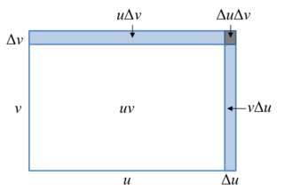
In the sense of definition 2, the equation ${\displaystyle \exp(x+y)=\exp(x)\exp(y)}$ follows from the term-by-term manipulation of power series justified by uniform convergence, and the resulting equality of coefficients is just the Binomial theorem. Furthermore: ^[1]

$${\displaystyle {\begin{aligned}\exp '(0)&=\lim _{h\to 0}{\frac {e^{h}-1}{h}}\\&=\lim _{h\to 0}{\frac {1}{h}}\left(\left(1+h+{\frac {h^{2}}{2!}}+{\frac {h^{3}}{3!}}+{\frac {h^{4}}{4!}}+\cdots \right)-1\right)\\&=\lim _{h\to 0}\left(1+{\frac {h}{2!}}+{\frac {h^{2}}{3!}}+{\frac {h^{3}}{4!}}+\cdots \right)\ =\ 1.\\\end{aligned}}}$$

Characterization 3 ⇔ characterization 4

Characterisation 3 involves defining the natural logarithm before the exponential function is defined. First,

$${\displaystyle \log x:=\int _{1}^{x}{\frac {dt}{t}}}$$

This means that the natural logarithm of ${\displaystyle x}$ equals the (signed) area under the graph of ${\displaystyle 1/t}$ between ${\displaystyle t=1}$ and ${\displaystyle t=x}$. If ${\displaystyle x<1}$, then this area is taken to be negative. Then, ${\displaystyle \exp }$ is defined as the inverse of ${\displaystyle \log }$, meaning that

$${\displaystyle \exp(\log(x))=x{\text{ and }}\log(\exp(x))=x}$$

by the definition of an inverse function. If ${\displaystyle a}$ is a positive real number then ${\displaystyle a^{x}}$ is defined as ${\displaystyle \exp(x\log(a))}$. Finally, ${\displaystyle e}$ is defined as the number ${\displaystyle a}$ such that ${\displaystyle \log(a)=1}$. It can then be shown that ${\displaystyle e^{x}=\exp(x)}$:

$${\displaystyle e^{x}=\exp(x\log(e))=\exp(x)}$$

By the fundamental theorem of calculus, the derivative of ${\textstyle \log x={\frac {1}{x}}}$. We are now in a position to prove that ${\textstyle {\frac {d}{dx}}e^{x}=e^{x}}$, satisfying the first part of the initial value problem given in characterisation 4:

$${\displaystyle {\begin{aligned}{\text{Let }}y&=e^{x}=\exp(x)\\\log(y)&=\log(\exp(x))=x\\{\frac {1}{y}}{\frac {dy}{dx}}&=1\\{\frac {dy}{dx}}&=y=e^{x}\end{aligned}}}$$

Then, we merely have to note that ${\displaystyle e^{0}=\exp(0)=1}$, and we are done. Of course, it is much easier to show that characterisation 4 implies characterisation 3. If ${\displaystyle e^{x}}$ is the unique function ${\displaystyle f:\mathbb {R} \to \mathbb {R} }$ satisfying ${\displaystyle f'(x)=e^{x}}$, and ${\displaystyle f(0)=1}$, then ${\displaystyle \log }$ can be defined as its inverse. The derivative of ${\displaystyle \log }$ can be found in the following way:

$${\displaystyle y=\log x\implies x=e^{y}}$$

If we differentiate both sides with respect to ${\displaystyle y}$, we get

$${\displaystyle {\begin{aligned}{\frac {dx}{dy}}&=e^{y}\\{\frac {dy}{dx}}&={\frac {1}{e^{y}}}={\frac {1}{x}}\end{aligned}}}$$

Therefore,

$${\displaystyle \int _{1}^{x}{\frac {1}{t}}dt=\left[\log t\right]_{1}^{x}=\log x-\log 1=\log x-0=\log x}$$

Characterization 5 ⇒ characterization 4

The conditions f'(0) = 1 and f(x + y) = f(x) f(y) imply both conditions in characterization 4. Indeed, one gets the initial condition f(0) = 1 by dividing both sides of the equation

$${\displaystyle f(0)=f(0+0)=f(0)f(0)}$$

by f(0), and the condition that f′(x) = f(x) follows from the condition that f′(0) = 1 and the definition of the derivative as follows:

$${\displaystyle {\begin{array}{rcccccc}f'(x)&=&\lim \limits _{h\to 0}{\frac {f(x+h)-f(x)}{h}}&=&\lim \limits _{h\to 0}{\frac {f(x)f(h)-f(x)}{h}}&=&\lim \limits _{h\to 0}f(x){\frac {f(h)-1}{h}}\\[1em]&=&f(x)\lim \limits _{h\to 0}{\frac {f(h)-1}{h}}&=&f(x)\lim \limits _{h\to 0}{\frac {f(0+h)-f(0)}{h}}&=&f(x)f'(0)=f(x).\end{array}}}$$

Characterization 5 ⇒ characterization 4

In the sense of definition 5, the multiplicative property together with the initial condition ${\displaystyle \exp '(0)=1}$ imply that:

$${\displaystyle {\begin{array}{rcl}{\frac {d}{dx}}\exp(x)&=&\lim _{h\to 0}{\frac {\exp(x{+}h)-\exp(x)}{h}}\\&=&\exp(x)\cdot \lim _{h\to 0}{\frac {\exp(h)-1}{h}}\\&=&\exp(x)\exp '(0)=\exp(x).\end{array}}}$$

Characterization 5 ⇔ characterization 6

The multiplicative property ${\displaystyle f(x+y)=f(x)f(y)}$ of definition 5 implies that ${\displaystyle f(0)=1}$, and that ${\displaystyle f(x)=a^{x}}$ according to the multiplication/division and root definition of exponentiation for rational ${\displaystyle x=n/m}$ in definition 6, where ${\displaystyle a=f(1)}$. Then the condition ${\displaystyle f'(0)=1}$ means that ${\displaystyle \lim _{h\to 0}{\tfrac {a^{h}-1}{h}}=1}$. Also any of the conditions of definition 5 imply that ${\displaystyle f(x)}$ is continuous at all real ${\displaystyle x}$. The converse is similar.

References

1. "Herman Yeung - Calculus - First Principle find d/Dx(e^x) 基本原理求 d/Dx(e^x)". YouTube .

• Walter Rudin, Principles of Mathematical Analysis, 3rd edition (McGraw–Hill, 1976), chapter 8.
• Edwin Hewitt and Karl Stromberg, Real and Abstract Analysis (Springer, 1965).