All non-isomorphic graphs on 3 vertices and their chromatic polynomials, clockwise from the top. The independent 3-set: k. An edge and a single vertex: k (k – 1). The 3-path: k(k – 1). The 3-clique: k(k – 1)(k – 2).
George David Birkhoff introduced the chromatic polynomial in 1912, defining it only for planar graphs, in an attempt to prove the four color theorem. If denotes the number of proper colorings of G with k colors then one could establish the four color theorem by showing for all planar graphs G. In this way he hoped to apply the powerful tools of analysis and algebra for studying the roots of polynomials to the combinatorial coloring problem.
Hassler Whitney generalised Birkhoff’s polynomial from the planar case to general graphs in 1932. In 1968, Ronald C. Read asked which polynomials are the chromatic polynomials of some graph, a question that remains open, and introduced the concept of chromatically equivalent graphs.[1] Today, chromatic polynomials are one of the central objects of algebraic graph theory.[2]
Definition
All proper vertex colorings of vertex graphs with 3 vertices using k colors for . The chromatic polynomial of each graph interpolates through the number of proper colorings.
For a graph G, counts the number of its (proper) vertex k-colorings. Other commonly used notations include , , or . There is a unique polynomial which evaluated at any integer k ≥ 0 coincides with ; it is called the chromatic polynomial of G.
For example, to color the path graph on 3 vertices with k colors, one may choose any of the k colors for the first vertex, any of the remaining colors for the second vertex, and lastly for the third vertex, any of the colors that are different from the second vertex's choice. Therefore, is the number of k-colorings of . For a variable x (not necessarily integer), we thus have . (Colorings which differ only by permuting colors or by automorphisms of G are still counted as different.)
The fact that the number of k-colorings is a polynomial in k follows from a recurrence relation called the deletion–contraction recurrence or Fundamental Reduction Theorem.[3] It is based on edge contraction: for a pair of vertices and the graph is obtained by merging the two vertices and removing any edges between them. If and are adjacent in G, let denote the graph obtained by removing the edge . Then the numbers of k-colorings of these graphs satisfy:
Equivalently, if and are not adjacent in G and is the graph with the edge added, then
This follows from the observation that every k-coloring of G either gives different colors to and , or the same colors. In the first case this gives a (proper) k-coloring of , while in the second case it gives a coloring of . Conversely, every k-coloring of G can be uniquely obtained from a k-coloring of or (if and are not adjacent in G).
The chromatic polynomial can hence be recursively defined as
for the edgeless graph on n vertices, and
for a graph G with an edge (arbitrarily chosen).
Since the number of k-colorings of the edgeless graph is indeed , it follows by induction on the number of edges that for all G, the polynomial coincides with the number of k-colorings at every integer point x=k. In particular, the chromatic polynomial is the unique interpolating polynomial of degree at most n through the points
Tutte’s curiosity about which other graph invariants satisfied such recurrences led him to discover a bivariate generalization of the chromatic polynomial, the Tutte polynomial.
For fixed G on n vertices, the chromatic polynomial is a monic polynomial of degree exactly n, with integer coefficients.
The chromatic polynomial includes at least as much information about the colorability of G as does the chromatic number. Indeed, the chromatic number is the smallest positive integer that is not a zero of the chromatic polynomial,
The polynomial evaluated at , that is , yields times the number of acyclic orientations of G.[4]
The coefficients of are all non-zero and alternate in signs.
The coefficient of is 1 (the polynomial is monic).
The coefficient of is
We prove this via induction on the number of edges on a simple graph G with vertices and edges. When , G is an empty graph. Hence per definition . So the coefficient of is , which implies the statement is true for an empty graph. When , as in G has just a single edge, . Thus coefficient of is . So the statement holds for k = 1. Using strong induction assume the statement is true for . Let G have edges. By the contraction-deletion principle,
Let and Hence . Since is obtained from G by removal of just one edge e, , so and thus the statement is true for k.
The coefficient of is times the number of acyclic orientations that have a unique sink, at a specified, arbitrarily chosen vertex.[5]
The absolute values of coefficients of every chromatic polynomial form a log-concave sequence.[6]
The last property is generalized by the fact that if G is a k-clique-sum of and (i.e., a graph obtained by gluing the two at a clique on k vertices), then
A graph G with n vertices is a tree if and only if
Chromatic equivalence
The three graphs with a chromatic polynomial equal to .
Two graphs are said to be chromatically equivalent if they have the same chromatic polynomial. Isomorphic graphs have the same chromatic polynomial, but non-isomorphic graphs can be chromatically equivalent. For example, all trees on n vertices have the same chromatic polynomial. In particular, is the chromatic polynomial of both the claw graph and the path graph on 4 vertices.
A graph is chromatically unique if it is determined by its chromatic polynomial, up to isomorphism. In other words, G is chromatically unique, then would imply that G and H are isomorphic. All cycle graphs are chromatically unique.[7]
Chromatic roots
A root (or zero) of a chromatic polynomial, called a “chromatic root”, is a value x where . Chromatic roots have been very well studied, in fact, Birkhoff’s original motivation for defining the chromatic polynomial was to show that for planar graphs, for x ≥ 4. This would have established the four color theorem.
No graph can be 0-colored, so 0 is always a chromatic root. Only edgeless graphs can be 1-colored, so 1 is a chromatic root of every graph with at least one edge. On the other hand, except for these two points, no graph can have a chromatic root at a real number smaller than or equal to 32/27.[8] A result of Tutte connects the golden ratio with the study of chromatic roots, showing that chromatic roots exist very close to : If is a planar triangulation of a sphere then
While the real line thus has large parts that contain no chromatic roots for any graph, every point in the complex plane is arbitrarily close to a chromatic root in the sense that there exists an infinite family of graphs whose chromatic roots are dense in the complex plane.[9]
Colorings using all colors
For a graph G on n vertices, let denote the number of colorings using exactly k colors up to renaming colors (so colorings that can be obtained from one another by permuting colors are counted as one; colorings obtained by automorphisms of G are still counted separately). In other words, counts the number of partitions of the vertex set into k (non-empty) independent sets. Then counts the number of colorings using exactly k colors (with distinguishable colors). For an integer x, all x-colorings of G can be uniquely obtained by choosing an integer k ≤ x, choosing k colors to be used out of x available, and a coloring using exactly those k (distinguishable) colors. Therefore:
where denotes the falling factorial. Thus the numbers are the coefficients of the polynomial in the basis of falling factorials.
Let be the k-th coefficient of in the standard basis , that is:
Computational problems associated with the chromatic polynomial include
finding the chromatic polynomial of a given graph G;
evaluating at a fixed x for given G.
The first problem is more general because if we knew the coefficients of we could evaluate it at any point in polynomial time because the degree is n. The difficulty of the second type of problem depends strongly on the value of x and has been intensively studied in computational complexity. When x is a natural number, this problem is normally viewed as computing the number of x-colorings of a given graph. For example, this includes the problem #3-coloring of counting the number of 3-colorings, a canonical problem in the study of complexity of counting, complete for the counting class #P.
Efficient algorithms
For some basic graph classes, closed formulas for the chromatic polynomial are known. For instance this is true for trees and cliques, as listed in the table above.
The deletion-contraction recurrence gives a way of computing the chromatic polynomial, called the deletion–contraction algorithm. In the first form (with a minus), the recurrence terminates in a collection of empty graphs. In the second form (with a plus), it terminates in a collection of complete graphs. This forms the basis of many algorithms for graph coloring. The ChromaticPolynomial function in the Combinatorica package of the computer algebra system Mathematica uses the second recurrence if the graph is dense, and the first recurrence if the graph is sparse.[13] The worst case running time of either formula satisfies the same recurrence relation as the Fibonacci numbers, so in the worst case, the algorithm runs in time within a polynomial factor of
on a graph with n vertices and m edges.[14] The analysis can be improved to within a polynomial factor of the number of spanning trees of the input graph.[15] In practice, branch and bound strategies and graph isomorphism rejection are employed to avoid some recursive calls, the running time depends on the heuristic used to pick the vertex pair.
Cube method
There is a natural geometric perspective on graph colorings by observing that, as an assignment of natural numbers to each vertex, a graph coloring is a vector in the integer lattice. Since two vertices and being given the same color is equivalent to the ’th and ’th coordinate in the coloring vector being equal, each edge can be associated with a hyperplane of the form . The collection of such hyperplanes for a given graph is called its graphic arrangement. The proper colorings of a graph are those lattice points which avoid forbidden hyperplanes. Restricting to a set of colors, the lattice points are contained in the cube . In this context the chromatic polynomial counts the number of lattice points in the -cube that avoid the graphic arrangement.
Computational complexity
The problem of computing the number of 3-colorings of a given graph is a canonical example of a #P-complete problem, so the problem of computing the coefficients of the chromatic polynomial is #P-hard. Similarly, evaluating for given G is #P-complete. On the other hand, for it is easy to compute , so the corresponding problems are polynomial-time computable. For integers the problem is #P-hard, which is established similar to the case . In fact, it is known that is #P-hard for all x (including negative integers and even all complex numbers) except for the three “easy points”.[16] Thus, from the perspective of #P-hardness, the complexity of computing the chromatic polynomial is completely understood.
In the expansion
the coefficient is always equal to 1, and several other properties of the coefficients are known. This raises the question if some of the coefficients are easy to compute. However the computational problem of computing ar for a fixed r ≥ 1 and a given graph G is #P-hard, even for bipartite planar graphs.[17]
No approximation algorithms for computing are known for any x except for the three easy points. At the integer points , the corresponding decision problem of deciding if a given graph can be k-colored is NP-hard. Such problems cannot be approximated to any multiplicative factor by a bounded-error probabilistic algorithm unless NP=RP, because any multiplicative approximation would distinguish the values 0 and 1, effectively solving the decision version in bounded-error probabilistic polynomial time. In particular, under the same assumption, this rules out the possibility of a fully polynomial time randomised approximation scheme (FPRAS). For other points, more complicated arguments are needed, and the question is the focus of active research. As of 2008[update], it is known that there is no FPRAS for computing for any x > 2, unless NP=RP holds.[18]
In graph theory, the girth of an undirected graph is the length of a shortest cycle contained in the graph. If the graph does not contain any cycles, its girth is defined to be infinity. For example, a 4-cycle (square) has girth 4. A grid has girth 4 as well, and a triangular mesh has girth 3. A graph with girth four or more is triangle-free.
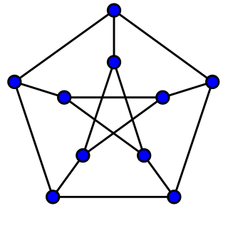
In the mathematical field of graph theory, the Petersen graph is an undirected graph with 10 vertices and 15 edges. It is a small graph that serves as a useful example and counterexample for many problems in graph theory. The Petersen graph is named after Julius Petersen, who in 1898 constructed it to be the smallest bridgeless cubic graph with no three-edge-coloring.
In graph theory, graph coloring is a special case of graph labeling; it is an assignment of labels traditionally called "colors" to elements of a graph subject to certain constraints. In its simplest form, it is a way of coloring the vertices of a graph such that no two adjacent vertices are of the same color; this is called a vertex coloring. Similarly, an edge coloring assigns a color to each edge so that no two adjacent edges are of the same color, and a face coloring of a planar graph assigns a color to each face or region so that no two faces that share a boundary have the same color.
In computer science, parameterized complexity is a branch of computational complexity theory that focuses on classifying computational problems according to their inherent difficulty with respect to multiple parameters of the input or output. The complexity of a problem is then measured as a function of those parameters. This allows the classification of NP-hard problems on a finer scale than in the classical setting, where the complexity of a problem is only measured as a function of the number of bits in the input. This appears to have been first demonstrated in Gurevich, Stockmeyer & Vishkin (1984). The first systematic work on parameterized complexity was done by Downey & Fellows (1999).
In graph theory, a perfect graph is a graph in which the chromatic number equals the size of the maximum clique, both in the graph itself and in every induced subgraph. In all graphs, the chromatic number is greater than or equal to the size of the maximum clique, but they can be far apart. A graph is perfect when these numbers are equal, and remain equal after the deletion of arbitrary subsets of vertices.
In the mathematical field of graph theory, a graph homomorphism is a mapping between two graphs that respects their structure. More concretely, it is a function between the vertex sets of two graphs that maps adjacent vertices to adjacent vertices.
In graph theory, a proper edge coloring of a graph is an assignment of "colors" to the edges of the graph so that no two incident edges have the same color. For example, the figure to the right shows an edge coloring of a graph by the colors red, blue, and green. Edge colorings are one of several different types of graph coloring. The edge-coloring problem asks whether it is possible to color the edges of a given graph using at most k different colors, for a given value of k, or with the fewest possible colors. The minimum required number of colors for the edges of a given graph is called the chromatic index of the graph. For example, the edges of the graph in the illustration can be colored by three colors but cannot be colored by two colors, so the graph shown has chromatic index three.
In graph theory, a branch of mathematics, list coloring is a type of graph coloring where each vertex can be restricted to a list of allowed colors. It was first studied in the 1970s in independent papers by Vizing and by Erdős, Rubin, and Taylor.
Fractional coloring is a topic in a young branch of graph theory known as fractional graph theory. It is a generalization of ordinary graph coloring. In a traditional graph coloring, each vertex in a graph is assigned some color, and adjacent vertices — those connected by edges — must be assigned different colors. In a fractional coloring however, a set of colors is assigned to each vertex of a graph. The requirement about adjacent vertices still holds, so if two vertices are joined by an edge, they must have no colors in common.
In graph theory, a graph property or graph invariant is a property of graphs that depends only on the abstract structure, not on graph representations such as particular labellings or drawings of the graph.
In graph theory, a domatic partition of a graph is a partition of into disjoint sets , ,..., such that each Vi is a dominating set for G. The figure on the right shows a domatic partition of a graph; here the dominating set consists of the yellow vertices, consists of the green vertices, and consists of the blue vertices.
The Tutte polynomial, also called the dichromate or the Tutte–Whitney polynomial, is a graph polynomial. It is a polynomial in two variables which plays an important role in graph theory. It is defined for every undirected graph and contains information about how the graph is connected. It is denoted by .
In the mathematical area of graph theory, Kőnig's theorem, proved by Dénes Kőnig, describes an equivalence between the maximum matching problem and the minimum vertex cover problem in bipartite graphs. It was discovered independently, also in 1931, by Jenő Egerváry in the more general case of weighted graphs.
In the mathematical area of graph theory, a triangle-free graph is an undirected graph in which no three vertices form a triangle of edges. Triangle-free graphs may be equivalently defined as graphs with clique number ≤ 2, graphs with girth ≥ 4, graphs with no induced 3-cycle, or locally independent graphs.
In graph theory, a nowhere-zero flow or NZ flow is a network flow that is nowhere zero. It is intimately connected to coloring planar graphs.
In the study of graph coloring problems in mathematics and computer science, a greedy coloring or sequential coloring is a coloring of the vertices of a graph formed by a greedy algorithm that considers the vertices of the graph in sequence and assigns each vertex its first available color. Greedy colorings can be found in linear time, but they do not, in general, use the minimum number of colors possible.
In the mathematical field of graph theory, the Chvátal graph is an undirected graph with 12 vertices and 24 edges, discovered by Václav Chvátal in 1970. It is the smallest graph that is triangle-free, 4-regular, and 4-chromatic.
In graph theory, a T-Coloring of a graph , given the set T of nonnegative integers containing 0, is a function that maps each vertex to a positive integer (color) such that if u and w are adjacent then . In simple words, the absolute value of the difference between two colors of adjacent vertices must not belong to fixed set T. The concept was introduced by William K. Hale. If T = {0} it reduces to common vertex coloring.
In graph theory, a mixed graphG = (V, E, A) is a graph consisting of a set of vertices V, a set of (undirected) edges E, and a set of directed edges (or arcs) A.
The order polynomial is a polynomial studied in mathematics, in particular in algebraic graph theory and algebraic combinatorics. The order polynomial counts the number of order-preserving maps from a poset to a chain of length . These order-preserving maps were first introduced by Richard P. Stanley while studying ordered structures and partitions as a Ph.D. student at Harvard University in 1971 under the guidance of Gian-Carlo Rota.
References
Biggs, N. (1993), Algebraic Graph Theory, Cambridge University Press, ISBN978-0-521-45897-9
Chao, C.-Y.; Whitehead, E. G. (1978), "On chromatic equivalence of graphs", Theory and Applications of Graphs, Lecture Notes in Mathematics, vol.642, Springer, pp.121–131, ISBN978-3-540-08666-6
Dong, F. M.; Koh, K. M.; Teo, K. L. (2005), Chromatic polynomials and chromaticity of graphs, World Scientific Publishing Company, ISBN978-981-256-317-0
Giménez, O.; Hliněný, P.; Noy, M. (2005), "Computing the Tutte polynomial on graphs of bounded clique-width", Proc. 31st Int. Worksh. Graph-Theoretic Concepts in Computer Science (WG 2005), Lecture Notes in Computer Science, vol.3787, Springer-Verlag, pp.59–68, CiteSeerX10.1.1.353.6385, doi:10.1007/11604686_6, ISBN978-3-540-31000-6
Jackson, B. (1993), "A Zero-Free Interval for Chromatic Polynomials of Graphs", Combinatorics, Probability and Computing, 2 (3): 325–336, doi:10.1017/S0963548300000705, S2CID39978844
Jaeger, F.; Vertigan, D. L.; Welsh, D. J. A. (1990), "On the computational complexity of the Jones and Tutte polynomials", Mathematical Proceedings of the Cambridge Philosophical Society, 108 (1): 35–53, Bibcode:1990MPCPS.108...35J, doi:10.1017/S0305004100068936, S2CID121454726
Linial, N. (1986), "Hard enumeration problems in geometry and combinatorics", SIAM J. Algebr. Discrete Methods, 7 (2): 331–335, doi:10.1137/0607036
Makowsky, J. A.; Rotics, U.; Averbouch, I.; Godlin, B. (2006), "Computing graph polynomials on graphs of bounded clique-width", Proc. 32nd Int. Worksh. Graph-Theoretic Concepts in Computer Science (WG 2006), Lecture Notes in Computer Science, vol.4271, Springer-Verlag, pp.191–204, CiteSeerX10.1.1.76.2320, doi:10.1007/11917496_18, ISBN978-3-540-48381-6
Naor, J.; Naor, M.; Schaffer, A. (1987), "Fast parallel algorithms for chordal graphs", Proc. 19th ACM Symp. Theory of Computing (STOC '87), pp.355–364, doi:10.1145/28395.28433, ISBN978-0897912211, S2CID12132229 .
Pemmaraju, S.; Skiena, S. (2003), Computational Discrete Mathematics: Combinatorics and Graph Theory with Mathematica, Cambridge University Press, section 7.4.2, ISBN978-0-521-80686-2
Sekine, Kyoko; Imai, Hiroshi; Tani, Seiichiro (1995), "Computing the Tutte polynomial of a graph of moderate size", in Staples, John; Eades, Peter; Katoh, Naoki; Moffat, Alistair (eds.), Algorithms and Computation, 6th International Symposium, ISAAC '95, Cairns, Australia, December 4–6, 1995, Proceedings, Lecture Notes in Computer Science, vol.1004, Springer, pp.224–233, doi:10.1007/BFb0015427
Code for computing Tutte, Chromatic and Flow Polynomials by Gary Haggard, David J. Pearce and Gordon Royle:
This page is based on this Wikipedia article Text is available under the CC BY-SA 4.0 license; additional terms may apply. Images, videos and audio are available under their respective licenses.