Branch and bound

Last updated

Branch and bound (BB, B&B, or BnB) is a method for solving optimization problems by breaking them down into smaller sub-problems and using a bounding function to eliminate sub-problems that cannot contain the optimal solution. It is an algorithm design paradigm for discrete and combinatorial optimization problems, as well as mathematical optimization. A branch-and-bound algorithm consists of a systematic enumeration of candidate solutions by means of state space search: the set of candidate solutions is thought of as forming a rooted tree with the full set at the root. The algorithm explores branches of this tree, which represent subsets of the solution set. Before enumerating the candidate solutions of a branch, the branch is checked against upper and lower estimated bounds on the optimal solution, and is discarded if it cannot produce a better solution than the best one found so far by the algorithm.

Contents

The algorithm depends on efficient estimation of the lower and upper bounds of regions/branches of the search space. If no bounds are available, the algorithm degenerates to an exhaustive search.

The method was first proposed by Ailsa Land and Alison Doig whilst carrying out research at the London School of Economics sponsored by British Petroleum in 1960 for discrete programming, [1] [2] and has become the most commonly used tool for solving NP-hard optimization problems. [3] The name "branch and bound" first occurred in the work of Little et al. on the traveling salesman problem. [4] [5]

Overview

The goal of a branch-and-bound algorithm is to find a value x that maximizes or minimizes the value of a real-valued function f(x), called an objective function, among some set S of admissible, or candidate solutions. The set S is called the search space, or feasible region. The rest of this section assumes that minimization of f(x) is desired; this assumption comes without loss of generality, since one can find the maximum value of f(x) by finding the minimum of g(x) = −f(x). A B&B algorithm operates according to two principles:

Turning these principles into a concrete algorithm for a specific optimization problem requires some kind of data structure that represents sets of candidate solutions. Such a representation is called an instance of the problem. Denote the set of candidate solutions of an instance I by SI. The instance representation has to come with three operations:

Using these operations, a B&B algorithm performs a top-down recursive search through the tree of instances formed by the branch operation. Upon visiting an instance I, it checks whether bound(I) is equal or greater than the current upper bound; if so, I may be safely discarded from the search and the recursion stops. This pruning step is usually implemented by maintaining a global variable that records the minimum upper bound seen among all instances examined so far.

Generic version

The following is the skeleton of a generic branch and bound algorithm for minimizing an arbitrary objective function f. [3] To obtain an actual algorithm from this, one requires a bounding function bound, that computes lower bounds of f on nodes of the search tree, as well as a problem-specific branching rule. As such, the generic algorithm presented here is a higher-order function.

  1. Using a heuristic, find a solution xh to the optimization problem. Store its value, B = f(xh). (If no heuristic is available, set B to infinity.) B will denote the best solution found so far, and will be used as an upper bound on candidate solutions.
  2. Initialize a queue to hold a partial solution with none of the variables of the problem assigned.
  3. Loop until the queue is empty:
    1. Take a node N off the queue.
    2. If N represents a single candidate solution x and f(x) < B, then x is the best solution so far. Record it and set Bf(x).
    3. Else, branch on N to produce new nodes Ni. For each of these:
      1. If bound(Ni) > B, do nothing; since the lower bound on this node is greater than the upper bound of the problem, it will never lead to the optimal solution, and can be discarded.
      2. Else, store Ni on the queue.

Several different queue data structures can be used. This FIFO queue-based implementation yields a breadth-first search. A stack (LIFO queue) will yield a depth-first algorithm. A best-first branch and bound algorithm can be obtained by using a priority queue that sorts nodes on their lower bound. [3] Examples of best-first search algorithms with this premise are Dijkstra's algorithm and its descendant A* search. The depth-first variant is recommended when no good heuristic is available for producing an initial solution, because it quickly produces full solutions, and therefore upper bounds. [7]

Pseudocode

A C++-like pseudocode implementation of the above is:

// C++-like implementation of branch and bound, // assuming the objective function f is to be minimizedCombinatorialSolutionbranch_and_bound_solve(CombinatorialProblemproblem,ObjectiveFunctionobjective_function/*f*/,BoundingFunctionlower_bound_function/*bound*/){// Step 1 abovedoubleproblem_upper_bound=std::numeric_limits<double>::infinity;// = BCombinatorialSolutionheuristic_solution=heuristic_solve(problem);// x_hproblem_upper_bound=objective_function(heuristic_solution);// B = f(x_h)CombinatorialSolutioncurrent_optimum=heuristic_solution;// Step 2 abovequeue<CandidateSolutionTree>candidate_queue;// problem-specific queue initializationcandidate_queue=populate_candidates(problem);while(!candidate_queue.empty()){// Step 3 above// Step 3.1CandidateSolutionTreenode=candidate_queue.pop();// "node" represents N aboveif(node.represents_single_candidate()){// Step 3.2if(objective_function(node.candidate())<problem_upper_bound){current_optimum=node.candidate();problem_upper_bound=objective_function(current_optimum);}// else, node is a single candidate which is not optimum}else{// Step 3.3: node represents a branch of candidate solutions// "child_branch" represents N_i abovefor(auto&&child_branch:node.candidate_nodes){if(lower_bound_function(child_branch)<=problem_upper_bound){candidate_queue.enqueue(child_branch);// Step 3.3.2}// otherwise, bound(N_i) > B so we prune the branch; step 3.3.1}}}returncurrent_optimum;}

In the above pseudocode, the functions heuristic_solve and populate_candidates called as subroutines must be provided as applicable to the problem. The functions f (objective_function) and bound (lower_bound_function) are treated as function objects as written, and could correspond to lambda expressions, function pointers and other types of callable objects in the C++ programming language.

Improvements

When is a vector of , branch and bound algorithms can be combined with interval analysis [8] and contractor techniques in order to provide guaranteed enclosures of the global minimum. [9] [10]

Applications

This approach is used for a number of NP-hard problems:

Branch-and-bound may also be a base of various heuristics. For example, one may wish to stop branching when the gap between the upper and lower bounds becomes smaller than a certain threshold. This is used when the solution is "good enough for practical purposes" and can greatly reduce the computations required. This type of solution is particularly applicable when the cost function used is noisy or is the result of statistical estimates and so is not known precisely but rather only known to lie within a range of values with a specific probability.[ citation needed ]

Relation to other algorithms

Nau et al. present a generalization of branch and bound that also subsumes the A*, B* and alpha-beta search algorithms. [16]

Optimization Example

Branch and bound can be used to solve this problem

Maximize with these constraints

and are integers.

The first step is to relax the integer constraint. We have two extreme points for the first equation that form a line: and . We can form the second line with the vector points and .

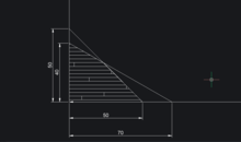
the two lines. Branch and Bound optimization example with linear constraints in BricsCad Ultimate Academic Edition.png
the two lines.

The third point is . This is a convex hull region so the solution lies on one of the vertices of the region. We can find the intersection using row reduction, which is , or with a value of 276.667. We test the other endpoints by sweeping the line over the region and find this is the maximum over the reals.

We choose the variable with the maximum fractional part, in this case becomes the parameter for the branch and bound method. We branch to and obtain 276 @ . We have reached an integer solution so we move to the other branch . We obtain 275.75 @. We have a decimal so we branch to and we find 274.571 @. We try the other branch and there are no feasible solutions. Therefore, the maximum is 276 with and .

See also

Related Research Articles

<span class="mw-page-title-main">Travelling salesman problem</span> NP-hard problem in combinatorial optimization

The travelling salesman problem, also known as the travelling salesperson problem (TSP), asks the following question: "Given a list of cities and the distances between each pair of cities, what is the shortest possible route that visits each city exactly once and returns to the origin city?" It is an NP-hard problem in combinatorial optimization, important in theoretical computer science and operations research.

<span class="mw-page-title-main">Linear programming</span> Method to solve optimization problems

Linear programming (LP), also called linear optimization, is a method to achieve the best outcome in a mathematical model whose requirements and objective are represented by linear relationships. Linear programming is a special case of mathematical programming.

<span class="mw-page-title-main">Mathematical optimization</span> Study of mathematical algorithms for optimization problems

Mathematical optimization or mathematical programming is the selection of a best element, with regard to some criterion, from some set of available alternatives. It is generally divided into two subfields: discrete optimization and continuous optimization. Optimization problems arise in all quantitative disciplines from computer science and engineering to operations research and economics, and the development of solution methods has been of interest in mathematics for centuries.

<span class="mw-page-title-main">Greedy algorithm</span> Sequence of locally optimal choices

A greedy algorithm is any algorithm that follows the problem-solving heuristic of making the locally optimal choice at each stage. In many problems, a greedy strategy does not produce an optimal solution, but a greedy heuristic can yield locally optimal solutions that approximate a globally optimal solution in a reasonable amount of time.

A* is a graph traversal and pathfinding algorithm, which is used in many fields of computer science due to its completeness, optimality, and optimal efficiency. Given a weighted graph, a source node and a goal node, the algorithm finds the shortest path from source to goal.

An integer programming problem is a mathematical optimization or feasibility program in which some or all of the variables are restricted to be integers. In many settings the term refers to integer linear programming (ILP), in which the objective function and the constraints are linear.

<span class="mw-page-title-main">Combinatorial optimization</span> Subfield of mathematical optimization

Combinatorial optimization is a subfield of mathematical optimization that consists of finding an optimal object from a finite set of objects, where the set of feasible solutions is discrete or can be reduced to a discrete set. Typical combinatorial optimization problems are the travelling salesman problem ("TSP"), the minimum spanning tree problem ("MST"), and the knapsack problem. In many such problems, such as the ones previously mentioned, exhaustive search is not tractable, and so specialized algorithms that quickly rule out large parts of the search space or approximation algorithms must be resorted to instead.

Global optimization is a branch of applied mathematics and numerical analysis that attempts to find the global minima or maxima of a function or a set of functions on a given set. It is usually described as a minimization problem because the maximization of the real-valued function is equivalent to the minimization of the function .

Iterative deepening A* (IDA*) is a graph traversal and path search algorithm that can find the shortest path between a designated start node and any member of a set of goal nodes in a weighted graph. It is a variant of iterative deepening depth-first search that borrows the idea to use a heuristic function to conservatively estimate the remaining cost to get to the goal from the A* search algorithm. Since it is a depth-first search algorithm, its memory usage is lower than in A*, but unlike ordinary iterative deepening search, it concentrates on exploring the most promising nodes and thus does not go to the same depth everywhere in the search tree. Unlike A*, IDA* does not utilize dynamic programming and therefore often ends up exploring the same nodes many times.

Branch and cut is a method of combinatorial optimization for solving integer linear programs (ILPs), that is, linear programming (LP) problems where some or all the unknowns are restricted to integer values. Branch and cut involves running a branch and bound algorithm and using cutting planes to tighten the linear programming relaxations. Note that if cuts are only used to tighten the initial LP relaxation, the algorithm is called cut and branch.

In mathematical optimization theory, duality or the duality principle is the principle that optimization problems may be viewed from either of two perspectives, the primal problem or the dual problem. If the primal is a minimization problem then the dual is a maximization problem. Any feasible solution to the primal (minimization) problem is at least as large as any feasible solution to the dual (maximization) problem. Therefore, the solution to the primal is an upper bound to the solution of the dual, and the solution of the dual is a lower bound to the solution of the primal. This fact is called weak duality.

In mathematical optimization, constrained optimization is the process of optimizing an objective function with respect to some variables in the presence of constraints on those variables. The objective function is either a cost function or energy function, which is to be minimized, or a reward function or utility function, which is to be maximized. Constraints can be either hard constraints, which set conditions for the variables that are required to be satisfied, or soft constraints, which have some variable values that are penalized in the objective function if, and based on the extent that, the conditions on the variables are not satisfied.

In mathematical optimization and related fields, relaxation is a modeling strategy. A relaxation is an approximation of a difficult problem by a nearby problem that is easier to solve. A solution of the relaxed problem provides information about the original problem.

<span class="mw-page-title-main">Linear programming relaxation</span>

In mathematics, the relaxation of a (mixed) integer linear program is the problem that arises by removing the integrality constraint of each variable.

<span class="mw-page-title-main">Feasible region</span> Mathematical constraints that define ways of finding the best solution

In mathematical optimization and computer science, a feasible region,feasible set, or solution space is the set of all possible points of an optimization problem that satisfy the problem's constraints, potentially including inequalities, equalities, and integer constraints. This is the initial set of candidate solutions to the problem, before the set of candidates has been narrowed down.

In applied mathematics, branch and price is a method of combinatorial optimization for solving integer linear programming (ILP) and mixed integer linear programming (MILP) problems with many variables. The method is a hybrid of branch and bound and column generation methods.

Variable neighborhood search (VNS), proposed by Mladenović & Hansen in 1997, is a metaheuristic method for solving a set of combinatorial optimization and global optimization problems. It explores distant neighborhoods of the current incumbent solution, and moves from there to a new one if and only if an improvement was made. The local search method is applied repeatedly to get from solutions in the neighborhood to local optima. VNS was designed for approximating solutions of discrete and continuous optimization problems and according to these, it is aimed for solving linear program problems, integer program problems, mixed integer program problems, nonlinear program problems, etc.

The quadratic knapsack problem (QKP), first introduced in 19th century, is an extension of knapsack problem that allows for quadratic terms in the objective function: Given a set of items, each with a weight, a value, and an extra profit that can be earned if two items are selected, determine the number of items to include in a collection without exceeding capacity of the knapsack, so as to maximize the overall profit. Usually, quadratic knapsack problems come with a restriction on the number of copies of each kind of item: either 0, or 1. This special type of QKP forms the 0-1 quadratic knapsack problem, which was first discussed by Gallo et al. The 0-1 quadratic knapsack problem is a variation of knapsack problems, combining the features of unbounded knapsack problem, 0-1 knapsack problem and quadratic knapsack problem.

ANTIGONE, is a deterministic global optimization solver for general Mixed-Integer Nonlinear Programs (MINLP).

In computer science, multiway number partitioning is the problem of partitioning a multiset of numbers into a fixed number of subsets, such that the sums of the subsets are as similar as possible. It was first presented by Ronald Graham in 1969 in the context of the identical-machines scheduling problem. The problem is parametrized by a positive integer k, and called k-way number partitioning. The input to the problem is a multiset S of numbers, whose sum is k*T.

References

  1. A. H. Land and A. G. Doig (1960). "An automatic method of solving discrete programming problems". Econometrica. 28 (3): 497–520. doi:10.2307/1910129. JSTOR   1910129.
  2. "Staff News". www.lse.ac.uk. Archived from the original on 2021-02-24. Retrieved 2018-10-08.
  3. 1 2 3 Clausen, Jens (1999). Branch and Bound Algorithms—Principles and Examples (PDF) (Technical report). University of Copenhagen. Archived from the original (PDF) on 2015-09-23. Retrieved 2014-08-13.
  4. 1 2 Little, John D. C.; Murty, Katta G.; Sweeney, Dura W.; Karel, Caroline (1963). "An algorithm for the traveling salesman problem" (PDF). Operations Research. 11 (6): 972–989. doi:10.1287/opre.11.6.972. hdl: 1721.1/46828 .
  5. Balas, Egon; Toth, Paolo (1983). Branch and bound methods for the traveling salesman problem (PDF) (Report). Carnegie Mellon University Graduate School of Industrial Administration. Archived (PDF) from the original on October 20, 2012.
  6. 1 2 Bader, David A.; Hart, William E.; Phillips, Cynthia A. (2004). "Parallel Algorithm Design for Branch and Bound" (PDF). In Greenberg, H. J. (ed.). Tutorials on Emerging Methodologies and Applications in Operations Research. Kluwer Academic Press. Archived from the original (PDF) on 2017-08-13. Retrieved 2015-09-16.
  7. Mehlhorn, Kurt; Sanders, Peter (2008). Algorithms and Data Structures: The Basic Toolbox (PDF). Springer. p. 249.
  8. Moore, R. E. (1966). Interval Analysis. Englewood Cliff, New Jersey: Prentice-Hall. ISBN   0-13-476853-1.
  9. Jaulin, L.; Kieffer, M.; Didrit, O.; Walter, E. (2001). Applied Interval Analysis. Berlin: Springer. ISBN   1-85233-219-0.
  10. Hansen, E.R. (1992). Global Optimization using Interval Analysis. New York: Marcel Dekker.
  11. Conway, Richard Walter; Maxwell, William L.; Miller, Louis W. (2003). Theory of Scheduling . Courier Dover Publications. pp.  56–61.
  12. Fukunaga, Keinosuke; Narendra, Patrenahalli M. (1975). "A branch and bound algorithm for computing k-nearest neighbors". IEEE Transactions on Computers (7): 750–753. doi:10.1109/t-c.1975.224297. S2CID   5941649.
  13. Narendra, Patrenahalli M.; Fukunaga, K. (1977). "A branch and bound algorithm for feature subset selection" (PDF). IEEE Transactions on Computers. C-26 (9): 917–922. doi:10.1109/TC.1977.1674939. S2CID   26204315.
  14. Hazimeh, Hussein; Mazumder, Rahul; Saab, Ali (2020). "Sparse Regression at Scale: Branch-and-Bound rooted in First-Order Optimization". arXiv: 2004.06152 [stat.CO].
  15. Nowozin, Sebastian; Lampert, Christoph H. (2011). "Structured Learning and Prediction in Computer Vision". Foundations and Trends in Computer Graphics and Vision. 6 (3–4): 185–365. CiteSeerX   10.1.1.636.2651 . doi:10.1561/0600000033. ISBN   978-1-60198-457-9.
  16. Nau, Dana S.; Kumar, Vipin; Kanal, Laveen (1984). "General branch and bound, and its relation to A∗ and AO∗" (PDF). Artificial Intelligence. 23 (1): 29–58. doi:10.1016/0004-3702(84)90004-3.