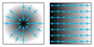
In vector calculus, the gradient of a scalar-valued differentiable function of several variables is the vector field whose value at a point is the "direction and rate of fastest increase". The gradient transforms like a vector under change of basis of the space of variables of . If the gradient of a function is non-zero at a point , the direction of the gradient is the direction in which the function increases most quickly from , and the magnitude of the gradient is the rate of increase in that direction, the greatest absolute directional derivative. Further, a point where the gradient is the zero vector is known as a stationary point. The gradient thus plays a fundamental role in optimization theory, where it is used to maximize a function by gradient ascent. In coordinate-free terms, the gradient of a function may be defined by:

The Navier–Stokes equations are partial differential equations which describe the motion of viscous fluid substances, named after French engineer and physicist Claude-Louis Navier and Irish physicist and mathematician George Gabriel Stokes. They were developed over several decades of progressively building the theories, from 1822 (Navier) to 1842–1850 (Stokes).
In the calculus of variations, a field of mathematical analysis, the functional derivative relates a change in a functional to a change in a function on which the functional depends.
In mathematics, the covariant derivative is a way of specifying a derivative along tangent vectors of a manifold. Alternatively, the covariant derivative is a way of introducing and working with a connection on a manifold by means of a differential operator, to be contrasted with the approach given by a principal connection on the frame bundle – see affine connection. In the special case of a manifold isometrically embedded into a higher-dimensional Euclidean space, the covariant derivative can be viewed as the orthogonal projection of the Euclidean directional derivative onto the manifold's tangent space. In this case the Euclidean derivative is broken into two parts, the extrinsic normal component and the intrinsic covariant derivative component.
In vector calculus, a conservative vector field is a vector field that is the gradient of some function. A conservative vector field has the property that its line integral is path independent; the choice of any path between two points does not change the value of the line integral. Path independence of the line integral is equivalent to the vector field under the line integral being conservative. A conservative vector field is also irrotational; in three dimensions, this means that it has vanishing curl. An irrotational vector field is necessarily conservative provided that the domain is simply connected.

A Halbach array is a special arrangement of permanent magnets that augments the magnetic field on one side of the array while cancelling the field to near zero on the other side. This is achieved by having a spatially rotating pattern of magnetisation.
In mathematics, the total variation identifies several slightly different concepts, related to the (local or global) structure of the codomain of a function or a measure. For a real-valued continuous function f, defined on an interval [a, b] ⊂ R, its total variation on the interval of definition is a measure of the one-dimensional arclength of the curve with parametric equation x ↦ f(x), for x ∈ [a, b]. Functions whose total variation is finite are called functions of bounded variation.
In physics and mathematics, in the area of vector calculus, Helmholtz's theorem, also known as the fundamental theorem of vector calculus, states that any sufficiently smooth, rapidly decaying vector field in three dimensions can be resolved into the sum of an irrotational (curl-free) vector field and a solenoidal (divergence-free) vector field; this is known as the Helmholtz decomposition or Helmholtz representation. It is named after Hermann von Helmholtz.
In optimization, the line search strategy is one of two basic iterative approaches to find a local minimum of an objective function . The other approach is trust region.
In (unconstrained) mathematical optimization, a backtracking line search is a line search method to determine the amount to move along a given search direction. Its use requires that the objective function is differentiable and that its gradient is known.
In numerical optimization, the Broyden–Fletcher–Goldfarb–Shanno (BFGS) algorithm is an iterative method for solving unconstrained nonlinear optimization problems. Like the related Davidon–Fletcher–Powell method, BFGS determines the descent direction by preconditioning the gradient with curvature information. It does so by gradually improving an approximation to the Hessian matrix of the loss function, obtained only from gradient evaluations via a generalized secant method.
One of the guiding principles in modern chemical dynamics and spectroscopy is that the motion of the nuclei in a molecule is slow compared to that of its electrons. This is justified by the large disparity between the mass of an electron, and the typical mass of a nucleus and leads to the Born–Oppenheimer approximation and the idea that the structure and dynamics of a chemical species are largely determined by nuclear motion on potential energy surfaces.
The Frank–Wolfe algorithm is an iterative first-order optimization algorithm for constrained convex optimization. Also known as the conditional gradient method, reduced gradient algorithm and the convex combination algorithm, the method was originally proposed by Marguerite Frank and Philip Wolfe in 1956. In each iteration, the Frank–Wolfe algorithm considers a linear approximation of the objective function, and moves towards a minimizer of this linear function.

In electromagnetism and applications, an inhomogeneous electromagnetic wave equation, or nonhomogeneous electromagnetic wave equation, is one of a set of wave equations describing the propagation of electromagnetic waves generated by nonzero source charges and currents. The source terms in the wave equations make the partial differential equations inhomogeneous, if the source terms are zero the equations reduce to the homogeneous electromagnetic wave equations. The equations follow from Maxwell's equations.
The gradient theorem, also known as the fundamental theorem of calculus for line integrals, says that a line integral through a gradient field can be evaluated by evaluating the original scalar field at the endpoints of the curve. The theorem is a generalization of the second fundamental theorem of calculus to any curve in a plane or space rather than just the real line.

The Navier–Stokes existence and smoothness problem concerns the mathematical properties of solutions to the Navier–Stokes equations, a system of partial differential equations that describe the motion of a fluid in space. Solutions to the Navier–Stokes equations are used in many practical applications. However, theoretical understanding of the solutions to these equations is incomplete. In particular, solutions of the Navier–Stokes equations often include turbulence, which remains one of the greatest unsolved problems in physics, despite its immense importance in science and engineering.
In applied mathematics, polyharmonic splines are used for function approximation and data interpolation. They are very useful for interpolating and fitting scattered data in many dimensions. Special cases include thin plate splines and natural cubic splines in one dimension.
There are various mathematical descriptions of the electromagnetic field that are used in the study of electromagnetism, one of the four fundamental interactions of nature. In this article, several approaches are discussed, although the equations are in terms of electric and magnetic fields, potentials, and charges with currents, generally speaking.
In differential calculus, there is no single uniform notation for differentiation. Instead, various notations for the derivative of a function or variable have been proposed by various mathematicians. The usefulness of each notation varies with the context, and it is sometimes advantageous to use more than one notation in a given context. The most common notations for differentiation are listed below.
Lagrangian field theory is a formalism in classical field theory. It is the field-theoretic analogue of Lagrangian mechanics. Lagrangian mechanics is used to analyze the motion of a system of discrete particles each with a finite number of degrees of freedom. Lagrangian field theory applies to continua and fields, which have an infinite number of degrees of freedom.


