Related Research Articles
In numerical analysis, Newton's method, also known as the Newton–Raphson method, named after Isaac Newton and Joseph Raphson, is a root-finding algorithm which produces successively better approximations to the roots of a real-valued function. The most basic version starts with a single-variable function f defined for a real variable x, the function's derivative f′, and an initial guess x0 for a root of f. If the function satisfies sufficient assumptions and the initial guess is close, then
Mathematical optimization or mathematical programming is the selection of a best element, with regard to some criterion, from some set of available alternatives. It is generally divided into two subfields: discrete optimization and continuous optimization. Optimization problems arise in all quantitative disciplines from computer science and engineering to operations research and economics, and the development of solution methods has been of interest in mathematics for centuries.
In mathematics and computing, a root-finding algorithm is an algorithm for finding zeros, also called "roots", of continuous functions. A zero of a function f, from the real numbers to real numbers or from the complex numbers to the complex numbers, is a number x such that f(x) = 0. As, generally, the zeros of a function cannot be computed exactly nor expressed in closed form, root-finding algorithms provide approximations to zeros, expressed either as floating-point numbers or as small isolating intervals, or disks for complex roots (an interval or disk output being equivalent to an approximate output together with an error bound).

In mathematics, a quadratic polynomial is a polynomial of degree two in one or more variables. A quadratic function is the polynomial function defined by a quadratic polynomial. Before 20th century, the distinction was unclear between a polynomial and its associated polynomial function; so "quadratic polynomial" and "quadratic function" were almost synonymous. This is still the case in many elementary courses, where both terms are often abbreviated as "quadratic".
In mathematics, the regula falsi, method of false position, or false position method is a very old method for solving an equation with one unknown; this method, in modified form, is still in use. In simple terms, the method is the trial and error technique of using test ("false") values for the variable and then adjusting the test value according to the outcome. This is sometimes also referred to as "guess and check". Versions of the method predate the advent of algebra and the use of equations.

The Gauss–Newton algorithm is used to solve non-linear least squares problems, which is equivalent to minimizing a sum of squared function values. It is an extension of Newton's method for finding a minimum of a non-linear function. Since a sum of squares must be nonnegative, the algorithm can be viewed as using Newton's method to iteratively approximate zeroes of the components of the sum, and thus minimizing the sum. In this sense, the algorithm is also an effective method for solving overdetermined systems of equations. It has the advantage that second derivatives, which can be challenging to compute, are not required.
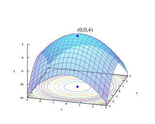
In calculus, Newton's method (also called Newton–Raphson) is an iterative method for finding the roots of a differentiable function F, which are solutions to the equation F (x) = 0. As such, Newton's method can be applied to the derivative f ′ of a twice-differentiable function f to find the roots of the derivative (solutions to f ′(x) = 0), also known as the critical points of f. These solutions may be minima, maxima, or saddle points; see section "Several variables" in Critical point (mathematics) and also section "Geometric interpretation" in this article. This is relevant in optimization, which aims to find (global) minima of the function f.
In numerical analysis, Brent's method is a hybrid root-finding algorithm combining the bisection method, the secant method and inverse quadratic interpolation. It has the reliability of bisection but it can be as quick as some of the less-reliable methods. The algorithm tries to use the potentially fast-converging secant method or inverse quadratic interpolation if possible, but it falls back to the more robust bisection method if necessary. Brent's method is due to Richard Brent and builds on an earlier algorithm by Theodorus Dekker. Consequently, the method is also known as the Brent–Dekker method.
In numerical analysis, inverse quadratic interpolation is a root-finding algorithm, meaning that it is an algorithm for solving equations of the form f(x) = 0. The idea is to use quadratic interpolation to approximate the inverse of f. This algorithm is rarely used on its own, but it is important because it forms part of the popular Brent's method.
For mathematical optimization, Multilevel Coordinate Search (MCS) is an efficient algorithm for bound constrained global optimization using function values only.

The Newton fractal is a boundary set in the complex plane which is characterized by Newton's method applied to a fixed polynomial p(Z) ∈ ℂ[Z] or transcendental function. It is the Julia set of the meromorphic function z ↦ z − p(z)/p′(z) which is given by Newton's method. When there are no attractive cycles (of order greater than 1), it divides the complex plane into regions Gk, each of which is associated with a root ζk of the polynomial, k = 1, …, deg(p). In this way the Newton fractal is similar to the Mandelbrot set, and like other fractals it exhibits an intricate appearance arising from a simple description. It is relevant to numerical analysis because it shows that (outside the region of quadratic convergence) the Newton method can be very sensitive to its choice of start point.
Simple rational approximation (SRA) is a subset of interpolating methods using rational functions. Especially, SRA interpolates a given function with a specific rational function whose poles and zeros are simple, which means that there is no multiplicity in poles and zeros. Sometimes, it only implies simple poles.
In numerical analysis, fixed-point iteration is a method of computing fixed points of a function.
Quasi-Newton methods are methods used to either find zeroes or local maxima and minima of functions, as an alternative to Newton's method. They can be used if the Jacobian or Hessian is unavailable or is too expensive to compute at every iteration. The "full" Newton's method requires the Jacobian in order to search for zeros, or the Hessian for finding extrema.
In numerical optimization, the nonlinear conjugate gradient method generalizes the conjugate gradient method to nonlinear optimization. For a quadratic function
Non-linear least squares is the form of least squares analysis used to fit a set of m observations with a model that is non-linear in n unknown parameters (m ≥ n). It is used in some forms of nonlinear regression. The basis of the method is to approximate the model by a linear one and to refine the parameters by successive iterations. There are many similarities to linear least squares, but also some significant differences. In economic theory, the non-linear least squares method is applied in (i) the probit regression, (ii) threshold regression, (iii) smooth regression, (iv) logistic link regression, (v) Box–Cox transformed regressors ().
In computational engineering, Luus–Jaakola (LJ) denotes a heuristic for global optimization of a real-valued function. In engineering use, LJ is not an algorithm that terminates with an optimal solution; nor is it an iterative method that generates a sequence of points that converges to an optimal solution. However, when applied to a twice continuously differentiable function, the LJ heuristic is a proper iterative method, that generates a sequence that has a convergent subsequence; for this class of problems, Newton's method is recommended and enjoys a quadratic rate of convergence, while no convergence rate analysis has been given for the LJ heuristic. In practice, the LJ heuristic has been recommended for functions that need be neither convex nor differentiable nor locally Lipschitz: The LJ heuristic does not use a gradient or subgradient when one be available, which allows its application to non-differentiable and non-convex problems.
Finding polynomial roots is a long-standing problem that has been the object of much research throughout history. A testament to this is that up until the 19th century, algebra meant essentially theory of polynomial equations.
References
Michael Heath (2002). Scientific Computing: An Introductory Survey (2nd ed.). New York: McGraw-Hill. ISBN 0-07-239910-4.
|  | |||||||||||||||||
|
| ||||||||||||||||||
| ||||||||||||||||||